57. Uncertainty Traps#
57.1. Overview#
In this lecture we study a simplified version of an uncertainty traps model of Fajgelbaum, Schaal and Taschereau-Dumouchel [FSTD15].
The model features self-reinforcing uncertainty that has big impacts on economic activity.
In the model,
Fundamentals vary stochastically and are not fully observable.
At any moment there are both active and inactive entrepreneurs; only active entrepreneurs produce.
Agents – active and inactive entrepreuneurs – have beliefs about the fundamentals expressed as probability distributions.
Greater uncertainty means greater dispersions of these distributions.
Entrepreneurs are risk averse and hence less inclined to be active when uncertainty is high.
The output of active entrepreneurs is observable, supplying a noisy signal that helps everyone inside the model infer fundamentals.
Entrepreneurs update their beliefs about fundamentals using Bayes’ Law, implemented via Kalman filtering.
Uncertainty traps emerge because:
High uncertainty discourages entrepreneurs from becoming active.
A low level of participation – i.e., a smaller number of active entrepreneurs – diminishes the flow of information about fundamentals.
Less information translates to higher uncertainty, further discouraging entrepreneurs from choosing to be active, and so on.
Uncertainty traps stem from a positive externality: high aggregate economic activity levels generates valuable information.
57.2. The Model#
The original model described in [FSTD15] has many interesting moving parts.
Here we examine a simplified version that nonetheless captures many of the key ideas.
57.2.1. Fundamentals#
The evolution of the fundamental process \(\{\theta_t\}\) is given by
where
\(\sigma_\theta > 0\) and \(0 < \rho < 1\)
\(\{w_t\}\) is IID and standard normal
The random variable \(\theta_t\) is not observable at any time.
57.2.2. Output#
There is a total \(\bar M\) of risk averse entrepreneurs.
Output of the \(m\)-th entrepreneur, conditional on being active in the market at time \(t\), is equal to
Here the time subscript has been dropped to simplify notation.
The inverse of the shock variance, \(\gamma_x\), is called the shock’s precision.
The higher is the precision, the more informative \(x_m\) is about the fundamental.
Output shocks are independent across time and firms.
57.2.3. Information and Beliefs#
All entrepreneurs start with identical beliefs about \(\theta_0\).
Signals are publicly observable and hence all agents have identical beliefs always.
Dropping time subscripts, beliefs for current \(\theta\) are represented by the normal distribution \(N(\mu, \gamma^{-1})\).
Here \(\gamma\) is the precision of beliefs; its inverse is the degree of uncertainty.
These parameters are updated by Kalman filtering.
Let
\(\mathbb M \subset \{1, \ldots, \bar M\}\) denote the set of currently active firms
\(M := |\mathbb M|\) denote the number of currently active firms
\(X\) be the average output \(\frac{1}{M} \sum_{m \in \mathbb M} x_m\) of the active firms
With this notation and primes for next period values, we can write the updating of the mean and precision via
These are standard Kalman filtering results applied to the current setting.
Exercise 1 provides more details on how (57.2) and (57.3) are derived, and then asks you to fill in remaining steps.
The next figure plots the law of motion for the precision in (57.3) as a 45 degree diagram, with one curve for each \(M \in \{0, \ldots, 6\}\).
The other parameter values are \(\rho = 0.99, \gamma_x = 0.5, \sigma_\theta =0.5\)
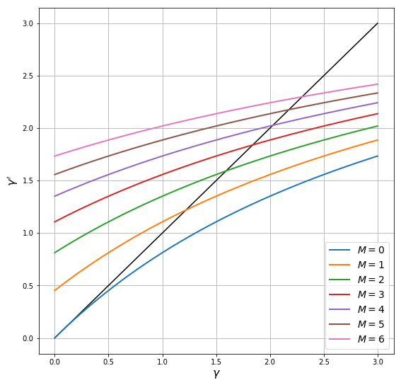
Points where the curves hit the 45 degree lines are long run steady states for precision for different values of \(M\).
Thus, if one of these values for \(M\) remains fixed, a corresponding steady state is the equilibrium level of precision
high values of \(M\) correspond to greater information about the fundamental, and hence more precision in steady state
low values of \(M\) correspond to less information and more uncertainty in steady state
In practice, as we’ll see, the number of active firms fluctuates stochastically.
57.2.4. Participation#
Omitting time subscripts once more, entrepreneurs enter the market in the current period if
Here
the mathematical expectation of \(x_m\) is based on (57.1) and beliefs \(N(\mu, \gamma^{-1})\) for \(\theta\)
\(F_m\) is a stochastic but previsible fixed cost, independent across time and firms
\(c\) is a constant reflecting opportunity costs
The statement that \(F_m\) is previsible means that it is realized at the start of the period and treated as a constant in (57.4).
The utility function has the constant absolute risk aversion form
where \(a\) is a positive parameter.
Combining (57.4) and (57.5), entrepreneur \(m\) participates in the market (or is said to be active) when
Using standard formulas for expectations of lognormal random variables, this is equivalent to the condition
57.3. Implementation#
We want to simulate this economy.
We’ll want a named tuple generator of the kind that we’ve seen before.
And we need methods to update \(\theta\), \(\mu\) and \(\gamma\), as well as to determine the number of active firms and their outputs.
The updating methods follow the laws of motion for \(\theta\), \(\mu\) and \(\gamma\) given above.
The method to evaluate the number of active firms generates \(F_1, \ldots, F_{\bar M}\) and tests condition (57.6) for each firm.
using Pkg; pkgs = ["DataFrames", "LaTeXStrings", "Plots"]; all(haskey.(Ref(Pkg.project().dependencies), pkgs)) || Pkg.add(pkgs)
using LinearAlgebra, Statistics
using DataFrames, LaTeXStrings, Plots
function # standard dev. of shock
UncertaintyTrapEcon(; a = 1.5,                       # risk aversion
                    gamma_x = 0.5,                  # production shock precision
                    rho = 0.99,                     # correlation coefficient for theta
                    sigma_theta = 0.5,              # standard dev. of theta shock
                    num_firms = 100,                # number of firms
                    sigma_F = 1.5,                  # standard dev. of fixed costs
                    c = -420.0,                     # external opportunity cost
                    mu_init = 0.0,                  # initial value for mu
                    gamma_init = 4.0,               # initial value for gamma
                    theta_init = 0.0,               # initial value for theta
                    sigma_x = sqrt(a / gamma_x)) # standard dev. of shock
    (; a, gamma_x, rho, sigma_theta, num_firms, sigma_F, c, mu_init, gamma_init,
     theta_init, sigma_x)
end
UncertaintyTrapEcon (generic function with 1 method)
In the results below we use this code to simulate time series for the major variables.
57.4. Results#
Let’s look first at the dynamics of \(\mu\), which the agents use to track \(\theta\)
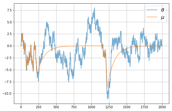
We see that \(\mu\) tracks \(\theta\) well when there are sufficient firms in the market.
However, there are times when \(\mu\) tracks \(\theta\) poorly due to insufficient information.
These are episodes where the uncertainty traps take hold.
During these episodes
precision is low and uncertainty is high
few firms are in the market
To get a clearer idea of the dynamics, let’s look at all the main time series at once, for a given set of shocks
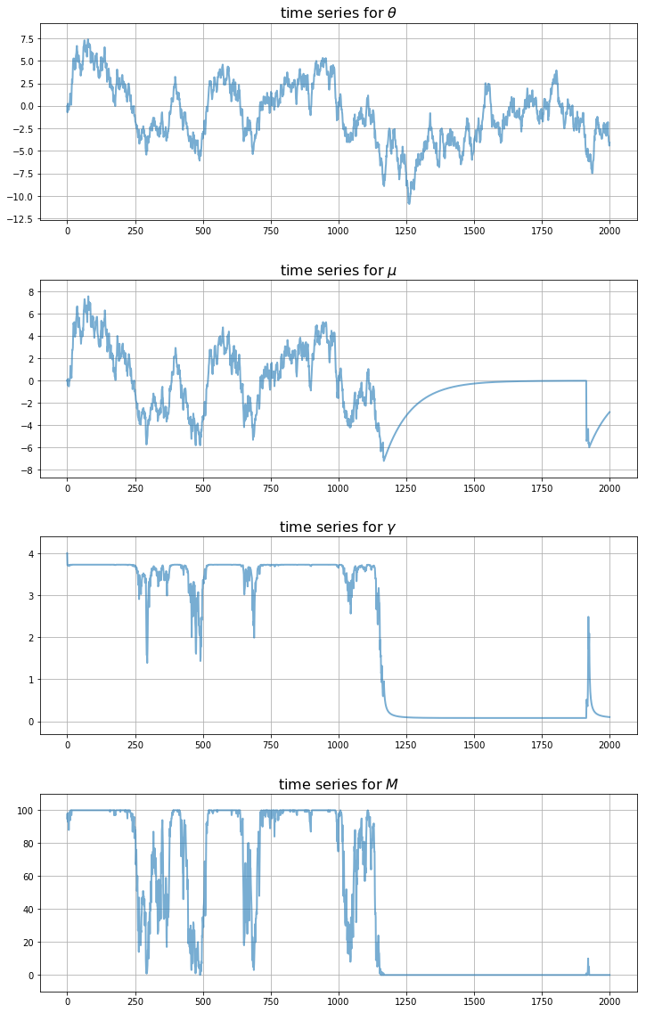
Notice how the traps only take hold after a sequence of bad draws for the fundamental.
Thus, the model gives us a propagation mechanism that maps bad random draws into long downturns in economic activity.
57.5. Exercises#
57.5.1. Exercise 1#
Fill in the details behind (57.2) and (57.3) based on the following standard result (see, e.g., p. 24 of [YS05]).
Fact Let \(\mathbf x = (x_1, \ldots, x_M)\) be a vector of IID draws from common distribution \(N(\theta, 1/\gamma_x)\) and let \(\bar x\) be the sample mean. If \(\gamma_x\) is known and the prior for \(\theta\) is \(N(\mu, 1/\gamma)\), then the posterior distribution of \(\theta\) given \(\mathbf x\) is
where
57.5.2. Exercise 2#
Modulo randomness, replicate the simulation figures shown above
Use the parameter values listed as defaults in the function UncertaintyTrapEcon.
57.6. Solutions#
57.6.1. Exercise 1#
This exercise asked you to validate the laws of motion for \(\gamma\) and \(\mu\) given in the lecture, based on the stated result about Bayesian updating in a scalar Gaussian setting.
The stated result tells us that after observing average output \(X\) of the \(M\) firms, our posterior beliefs will be
where
If we take a random variable \(\theta\) with this distribution and then evaluate the distribution of \(\rho \theta + \sigma_\theta w\) where \(w\) is independent and standard normal, we get the expressions for \(\mu'\) and \(\gamma'\) given in the lecture.
57.7. Exercise 2#
First let’s replicate the plot that illustrates the law of motion for precision, which is
Here \(M\) is the number of active firms. The next figure plots \(\gamma_{t+1}\) against \(\gamma_t\) on a 45 degree diagram for different values of \(M\)
econ = UncertaintyTrapEcon()
(; rho, sigma_theta, gamma_x) = econ # simplify names

# grid for gamma and gamma_{t+1}
gamma = range(1e-10, 3, length = 200)
M_range = 0:6
gammap = 1 ./ (rho^2 ./ (gamma .+ gamma_x .* M_range') .+ sigma_theta^2)

labels = ["0" "1" "2" "3" "4" "5" "6"]

plot(gamma, gamma, lw = 2, label = "45 Degree")
plot!(gamma, gammap, lw = 2, label = labels)
plot!(xlabel = L"\gamma", ylabel = L"\gamma^\prime", legend_title = L"M",
      legend = :bottomright)

The points where the curves hit the 45 degree lines are the long run steady states corresponding to each \(M\), if that value of \(M\) was to remain fixed. As the number of firms falls, so does the long run steady state of precision.
Next let’s generate time series for beliefs and the aggregates – that is, the number of active firms and average output
function simulate(uc, capT = 2_000)
    # unpack parameters
    (; a, gamma_x, rho, sigma_theta, num_firms, sigma_F, c, mu_init, gamma_init, theta_init, sigma_x) = uc

    # draw standard normal shocks
    w_shocks = randn(capT)

    # aggregate functions
    # auxiliary function psi
    function psi(gamma, mu, F)
        temp1 = -a * (mu - F)
        temp2 = 0.5 * a^2 / (gamma + gamma_x)
        return (1 - exp(temp1 + temp2)) / a - c
    end

    # compute X, M
    function gen_aggregates(gamma, mu, theta)
        F_vals = sigma_F * randn(num_firms)
        M = sum(psi.(Ref(gamma), Ref(mu), F_vals) .> 0) # counts number of active firms
        if any(psi(gamma, mu, f) > 0 for f in F_vals) # there is an active firm
            x_vals = theta .+ sigma_x * randn(M)
            X = mean(x_vals)
        else
            X = 0.0
        end
        return (; X, M)
    end

    # initialize dataframe
    X_init, M_init = gen_aggregates(gamma_init, mu_init, theta_init)
    df = DataFrame(gamma = gamma_init, mu = mu_init, theta = theta_init,
                   X = X_init, M = M_init)

    # update dataframe
    for t in 2:capT
        # unpack old variables
        theta_old, gamma_old, mu_old, X_old, M_old = (df.theta[end],
                                                      df.gamma[end], df.mu[end],
                                                      df.X[end], df.M[end])

        # define new beliefs
        theta = rho * theta_old + sigma_theta * w_shocks[t - 1]
        mu = (rho * (gamma_old * mu_old + M_old * gamma_x * X_old)) /
             (gamma_old + M_old * gamma_x)
        gamma = 1 / (rho^2 / (gamma_old + M_old * gamma_x) + sigma_theta^2)

        # compute new aggregates
        X, M = gen_aggregates(gamma, mu, theta)
        push!(df, (; gamma, mu, theta, X, M))
    end

    # return
    return df
end
simulate (generic function with 2 methods)
First let’s see how well \(\mu\) tracks \(\theta\) in these simulations
df = simulate(econ)

plot(eachindex(df.mu), df.mu, lw = 2, label = L"\mu")
plot!(eachindex(df.theta), df.theta, lw = 2, label = L"\theta")
plot!(xlabel = L"x", ylabel = L"y", legend_title = "Variable",
      legend = :bottomright)

Now let’s plot the whole thing together
len = eachindex(df.theta)
yvals = [df.theta, df.mu, df.gamma, df.M]
vars = [L"\theta", L"\mu", L"\gamma", L"M"]

plt = plot(layout = (4, 1), size = (600, 600))

for i in 1:4
    plot!(plt[i], len, yvals[i], xlabel = L"t", ylabel = vars[i], label = "")
end

plot(plt)
