24. Linear State Space Models #

Contents

Linear State Space Models

“We may regard the present state of the universe as the effect of its past and the cause of its future” – Marquis de Laplace

24.1. Overview #

This lecture introduces the linear state space dynamic system.

This model is a workhorse that carries a powerful theory of prediction.

Its many applications include:

representing dynamics of higher-order linear systems
predicting the position of a system \(j\) steps into the future
predicting a geometric sum of future values of a variable like
- non financial income
- dividends on a stock
- the money supply
- a government deficit or surplus, etc.
key ingredient of useful models
- Friedman’s permanent income model of consumption smoothing
- Barro’s model of smoothing total tax collections
- Rational expectations version of Cagan’s model of hyperinflation
- Sargent and Wallace’s “unpleasant monetarist arithmetic,” etc.

using LinearAlgebra, Statistics

24.2. The Linear State Space Model #

The objects in play are:

An \(n \times 1\) vector \(x_t\) denoting the state at time \(t = 0, 1, 2, \ldots\).
An iid sequence of \(m \times 1\) random vectors \(w_t \sim N(0,I)\).
A \(k \times 1\) vector \(y_t\) of observations at time \(t = 0, 1, 2, \ldots\).
An \(n \times n\) matrix \(A\) called the transition matrix.
An \(n \times m\) matrix \(C\) called the volatility matrix.
A \(k \times n\) matrix \(G\) sometimes called the output matrix.

Here is the linear state-space system

(24.1)#\[\begin{split}\begin{aligned} x_{t+1} & = A x_t + C w_{t+1} \\ y_t & = G x_t \nonumber \\ x_0 & \sim N(\mu_0, \Sigma_0) \nonumber \end{aligned}\end{split}\]

24.2.1. Primitives#

The primitives of the model are

the matrices \(A, C, G\)
shock distribution, which we have specialized to \(N(0,I)\)
the distribution of the initial condition \(x_0\), which we have set to \(N(\mu_0, \Sigma_0)\)

Given \(A, C, G\) and draws of \(x_0\) and \(w_1, w_2, \ldots\), the model (24.1) pins down the values of the sequences \(\{x_t\}\) and \(\{y_t\}\).

Even without these draws, the primitives 1–3 pin down the probability distributions of \(\{x_t\}\) and \(\{y_t\}\).

Later we’ll see how to compute these distributions and their moments.

24.2.1.1. Martingale difference shocks#

We’ve made the common assumption that the shocks are independent standardized normal vectors.

But some of what we say will be valid under the assumption that \(\{w_{t+1}\}\) is a martingale difference sequence.

A martingale difference sequence is a sequence that is zero mean when conditioned on past information.

In the present case, since \(\{x_t\}\) is our state sequence, this means that it satisfies

\[ \mathbb{E} [w_{t+1} | x_t, x_{t-1}, \ldots ] = 0 \]

This is a weaker condition than that \(\{w_t\}\) is iid with \(w_{t+1} \sim N(0,I)\).

24.2.2. Examples#

By appropriate choice of the primitives, a variety of dynamics can be represented in terms of the linear state space model.

The following examples help to highlight this point.

They also illustrate the wise dictum finding the state is an art.

24.2.2.1. Second-order difference equation#

Let \(\{y_t\}\) be a deterministic sequence that satisfies

(24.2)#\[y_{t+1} = \phi_0 + \phi_1 y_t + \phi_2 y_{t-1} \quad \text{s.t.} \quad y_0, y_{-1} \text{ given}\]

To map (24.2) into our state space system (24.1), we set

\[\begin{split} x_t= \begin{bmatrix} 1 \\ y_t \\ y_{t-1} \end{bmatrix} \qquad A = \begin{bmatrix} 1 & 0 & 0 \\ \phi_0 & \phi_1 & \phi_2 \\ 0 & 1 & 0 \end{bmatrix} \qquad C= \begin{bmatrix} 0 \\ 0 \\ 0 \end{bmatrix} \qquad G = \begin{bmatrix} 0 & 1 & 0 \end{bmatrix} \end{split}\]

You can confirm that under these definitions, (24.1) and (24.2) agree.

The next figure shows dynamics of this process when \(\phi_0 = 1.1, \phi_1=0.8, \phi_2 = -0.8, y_0 = y_{-1} = 1\)

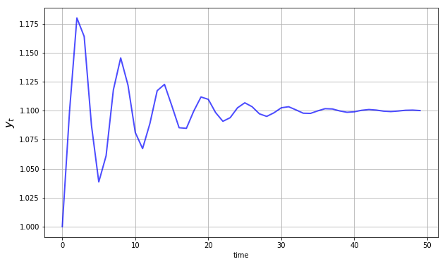
Later you’ll be asked to recreate this figure.

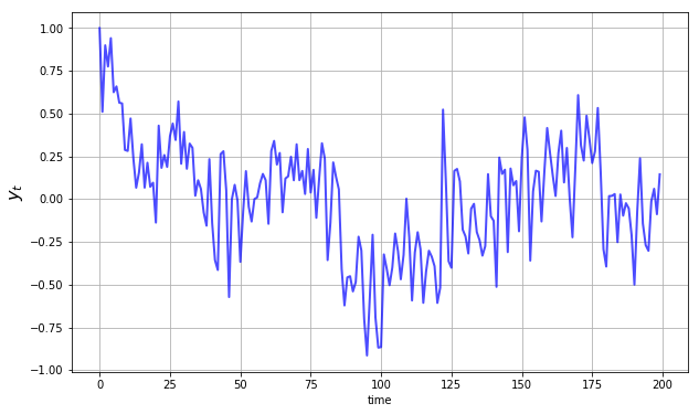
24.2.2.2. Univariate Autoregressive Processes#

We can use (24.1) to represent the model

(24.3)#\[y_{t+1} = \phi_1 y_{t} + \phi_2 y_{t-1} + \phi_3 y_{t-2} + \phi_4 y_{t-3} + \sigma w_{t+1}\]

where \(\{w_t\}\) is iid and standard normal.

To put this in the linear state space format we take \(x_t = \begin{bmatrix} y_t & y_{t-1} & y_{t-2} & y_{t-3} \end{bmatrix}'\) and

\[\begin{split} A = \begin{bmatrix} \phi_1 & \phi_2 & \phi_3 & \phi_4 \\ 1 & 0 & 0 & 0 \\ 0 & 1 & 0 & 0 \\ 0 & 0 & 1 & 0 \end{bmatrix} \qquad C = \begin{bmatrix} \sigma \\ 0 \\ 0 \\ 0 \end{bmatrix} \qquad G = \begin{bmatrix} 1 & 0 & 0 & 0 \end{bmatrix} \end{split}\]

The matrix \(A\) has the form of the companion matrix to the vector \(\begin{bmatrix}\phi_1 & \phi_2 & \phi_3 & \phi_4 \end{bmatrix}\).

The next figure shows dynamics of this process when

\[ \phi_1 = 0.5, \phi_2 = -0.2, \phi_3 = 0, \phi_4 = 0.5, \sigma = 0.2, y_0 = y_{-1} = y_{-2} = y_{-3} = 1 \]

24.2.2.3. Vector Autoregressions#

Now suppose that

\(y_t\) is a \(k \times 1\) vector
\(\phi_j\) is a \(k \times k\) matrix and
\(w_t\) is \(k \times 1\)

Then (24.3) is termed a vector autoregression.

To map this into (24.1), we set

\[\begin{split} x_t = \begin{bmatrix} y_t \\ y_{t-1} \\ y_{t-2} \\ y_{t-3} \end{bmatrix} \quad A = \begin{bmatrix} \phi_1 & \phi_2 & \phi_3 & \phi_4 \\ I & 0 & 0 & 0 \\ 0 & I & 0 & 0 \\ 0 & 0 & I & 0 \end{bmatrix} \quad C = \begin{bmatrix} \sigma \\ 0 \\ 0 \\ 0 \end{bmatrix} \quad G = \begin{bmatrix} I & 0 & 0 & 0 \end{bmatrix} \end{split}\]

where \(I\) is the \(k \times k\) identity matrix and \(\sigma\) is a \(k \times k\) matrix.

24.2.2.4. Seasonals#

We can use (24.1) to represent

the deterministic seasonal \(y_t = y_{t-4}\)
the indeterministic seasonal \(y_t = \phi_4 y_{t-4} + w_t\)

In fact both are special cases of (24.3).

With the deterministic seasonal, the transition matrix becomes

\[\begin{split} A = \begin{bmatrix} 0 & 0 & 0 & 1 \\ 1 & 0 & 0 & 0 \\ 0 & 1 & 0 & 0 \\ 0 & 0 & 1 & 0 \end{bmatrix} \end{split}\]

It is easy to check that \(A^4 = I\), which implies that \(x_t\) is strictly periodic with period 4:1

\[ x_{t+4} = x_t \]

Such an \(x_t\) process can be used to model deterministic seasonals in quarterly time series.

The indeterministic seasonal produces recurrent, but aperiodic, seasonal fluctuations.

24.2.2.5. Time Trends#

The model \(y_t = a t + b\) is known as a linear time trend.

We can represent this model in the linear state space form by taking

(24.4)#\[\begin{split}A = \begin{bmatrix} 1 & 1 \\ 0 & 1 \end{bmatrix} \qquad C = \begin{bmatrix} 0 \\ 0 \end{bmatrix} \qquad G = \begin{bmatrix} a & b \end{bmatrix}\end{split}\]

and starting at initial condition \(x_0 = \begin{bmatrix} 0 & 1\end{bmatrix}'\).

In fact it’s possible to use the state-space system to represent polynomial trends of any order.

For instance, let

\[\begin{split} x_0 = \begin{bmatrix} 0 \\ 0 \\ 1 \end{bmatrix} \qquad A = \begin{bmatrix} 1 & 1 & 0 \\ 0 & 1 & 1 \\ 0 & 0 & 1 \end{bmatrix} \qquad C = \begin{bmatrix} 0 \\ 0 \\ 0 \end{bmatrix} \end{split}\]

It follows that

\[\begin{split} A^t = \begin{bmatrix} 1 & t & t(t-1)/2 \\ 0 & 1 & t \\ 0 & 0 & 1 \end{bmatrix} \end{split}\]

Then \(x_t^\prime = \begin{bmatrix} t(t-1)/2 &t & 1 \end{bmatrix}\), so that \(x_t\) contains linear and quadratic time trends.

24.2.3. Moving Average Representations#

A nonrecursive expression for \(x_t\) as a function of \(x_0, w_1, w_2, \ldots, w_t\) can be found by using (24.1) repeatedly to obtain

(24.5)#\[\begin{split}\begin{aligned} x_t & = Ax_{t-1} + Cw_t \\ & = A^2 x_{t-2} + ACw_{t-1} + Cw_t \nonumber \\ & \qquad \vdots \nonumber \\ & = \sum_{j=0}^{t-1} A^j Cw_{t-j} + A^t x_0 \nonumber \end{aligned}\end{split}\]

Representation (24.5) is a moving average representation.

It expresses \(\{x_t\}\) as a linear function of

current and past values of the process \(\{w_t\}\) and
the initial condition \(x_0\)

As an example of a moving average representation, let the model be

\[\begin{split} A = \begin{bmatrix} 1 & 1 \\ 0 & 1 \end{bmatrix} \qquad C = \begin{bmatrix} 1 \\ 0 \end{bmatrix} \end{split}\]

You will be able to show that \(A^t = \begin{bmatrix} 1 & t \cr 0 & 1 \end{bmatrix}\) and \(A^j C = \begin{bmatrix} 1 & 0 \end{bmatrix}'\).

Substituting into the moving average representation (24.5), we obtain

\[ x_{1t} = \sum_{j=0}^{t-1} w_{t-j} + \begin{bmatrix} 1 & t \end{bmatrix} x_0 \]

where \(x_{1t}\) is the first entry of \(x_t\).

The first term on the right is a cumulated sum of martingale differences, and is therefore a martingale.

The second term is a translated linear function of time.

For this reason, \(x_{1t}\) is called a martingale with drift.

24.3. Distributions and Moments #

24.3.1. Unconditional Moments#

Using (24.1), it’s easy to obtain expressions for the (unconditional) means of \(x_t\) and \(y_t\).

We’ll explain what unconditional and conditional mean soon.

Letting \(\mu_t := \mathbb{E} [x_t]\) and using linearity of expectations, we find that

(24.6)#\[\mu_{t+1} = A \mu_t \quad \text{with} \quad \mu_0 \text{ given}\]

Here \(\mu_0\) is a primitive given in (24.1).

The variance-covariance matrix of \(x_t\) is \(\Sigma_t := \mathbb{E} [ (x_t - \mu_t) (x_t - \mu_t)']\).

Using \(x_{t+1} - \mu_{t+1} = A (x_t - \mu_t) + C w_{t+1}\), we can determine this matrix recursively via

(24.7)#\[\Sigma_{t+1} = A \Sigma_t A' + C C' \quad \text{with} \quad \Sigma_0 \text{ given}\]

As with \(\mu_0\), the matrix \(\Sigma_0\) is a primitive given in (24.1).

As a matter of terminology, we will sometimes call

\(\mu_t\) the unconditional mean of \(x_t\)
\(\Sigma_t\) the unconditional variance-convariance matrix of \(x_t\)

This is to distinguish \(\mu_t\) and \(\Sigma_t\) from related objects that use conditioning information, to be defined below.

However, you should be aware that these “unconditional” moments do depend on the initial distribution \(N(\mu_0, \Sigma_0)\).

24.3.1.1. Moments of the Observations#

Using linearity of expectations again we have

(24.8)#\[\mathbb{E} [y_t] = \mathbb{E} [G x_t] = G \mu_t\]

The variance-covariance matrix of \(y_t\) is easily shown to be

(24.9)#\[\textrm{Var} [y_t] = \textrm{Var} [G x_t] = G \Sigma_t G'\]

24.3.2. Distributions#

In general, knowing the mean and variance-covariance matrix of a random vector is not quite as good as knowing the full distribution.

However, there are some situations where these moments alone tell us all we need to know.

These are situations in which the mean vector and covariance matrix are sufficient statistics for the population distribution.

(Sufficient statistics form a list of objects that characterize a population distribution)

One such situation is when the vector in question is Gaussian (i.e., normally distributed).

This is the case here, given

our Gaussian assumptions on the primitives
the fact that normality is preserved under linear operations

In fact, it’s well-known that

(24.10)#\[u \sim N(\bar u, S) \quad \text{and} \quad v = a + B u \implies v \sim N(a + B \bar u, B S B')\]

In particular, given our Gaussian assumptions on the primitives and the linearity of (24.1) we can see immediately that both \(x_t\) and \(y_t\) are Gaussian for all \(t \geq 0\) 2.

Since \(x_t\) is Gaussian, to find the distribution, all we need to do is find its mean and variance-covariance matrix.

But in fact we’ve already done this, in (24.6) and (24.7).

Letting \(\mu_t\) and \(\Sigma_t\) be as defined by these equations, we have

(24.11)#\[x_t \sim N(\mu_t, \Sigma_t)\]

By similar reasoning combined with (24.8) and (24.9),

(24.12)#\[y_t \sim N(G \mu_t, G \Sigma_t G')\]

24.3.3. Ensemble Interpretations#

How should we interpret the distributions defined by (24.11)–(24.12)?

Intuitively, the probabilities in a distribution correspond to relative frequencies in a large population drawn from that distribution.

Let’s apply this idea to our setting, focusing on the distribution of \(y_T\) for fixed \(T\).

We can generate independent draws of \(y_T\) by repeatedly simulating the evolution of the system up to time \(T\), using an independent set of shocks each time.

The next figure shows 20 simulations, producing 20 time series for \(\{y_t\}\), and hence 20 draws of \(y_T\).

The system in question is the univariate autoregressive model (24.3).

The values of \(y_T\) are represented by black dots in the left-hand figure

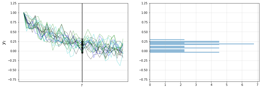
In the right-hand figure, these values are converted into a rotated histogram that shows relative frequencies from our sample of 20 \(y_T\)’s.

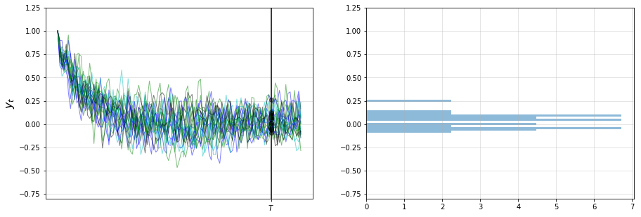
(The parameters and source code for the figures can be found in file linear_models/paths_and_hist.jl)

Here is another figure, this time with 100 observations

Let’s now try with 500,000 observations, showing only the histogram (without rotation)

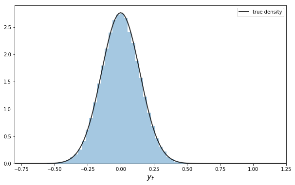
The black line is the population density of \(y_T\) calculated from (24.12).

The histogram and population distribution are close, as expected.

By looking at the figures and experimenting with parameters, you will gain a feel for how the population distribution depends on the model primitives listed above, as intermediated by the distribution’s sufficient statistics.

24.3.3.1. Ensemble means#

In the preceding figure we approximated the population distribution of \(y_T\) by

generating \(I\) sample paths (i.e., time series) where \(I\) is a large number
recording each observation \(y^i_T\)
histogramming this sample

Just as the histogram approximates the population distribution, the ensemble or cross-sectional average

\[ \bar y_T := \frac{1}{I} \sum_{i=1}^I y_T^i \]

approximates the expectation \(\mathbb{E} [y_T] = G \mu_T\) (as implied by the law of large numbers).

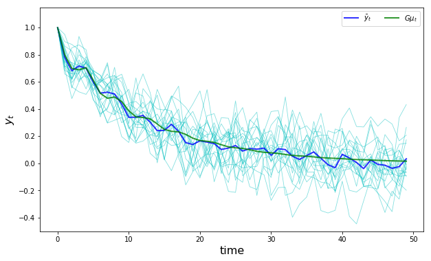
Here’s a simulation comparing the ensemble averages and population means at time points \(t=0,\ldots,50\).

The parameters are the same as for the preceding figures, and the sample size is relatively small (\(I=20\)).

The ensemble mean for \(x_t\) is

\[ \bar x_T := \frac{1}{I} \sum_{i=1}^I x_T^i \to \mu_T \qquad (I \to \infty) \]

The limit \(\mu_T\) is a “long-run average”.

(By long-run average we mean the average for an infinite (\(I = \infty\)) number of sample \(x_T\)’s)

Another application of the law of large numbers assures us that

\[ \frac{1}{I} \sum_{i=1}^I (x_T^i - \bar x_T) (x_T^i - \bar x_T)' \to \Sigma_T \qquad (I \to \infty) \]

24.3.4. Joint Distributions#

In the preceding discussion we looked at the distributions of \(x_t\) and \(y_t\) in isolation.

This gives us useful information, but doesn’t allow us to answer questions like

what’s the probability that \(x_t \geq 0\) for all \(t\)?
what’s the probability that the process \(\{y_t\}\) exceeds some value \(a\) before falling below \(b\)?
etc., etc.

Such questions concern the joint distributions of these sequences.

To compute the joint distribution of \(x_0, x_1, \ldots, x_T\), recall that joint and conditional densities are linked by the rule

\[ p(x, y) = p(y \, | \, x) p(x) \qquad \text{(joint }=\text{ conditional }\times\text{ marginal)} \]

From this rule we get \(p(x_0, x_1) = p(x_1 \,|\, x_0) p(x_0)\).

The Markov property \(p(x_t \,|\, x_{t-1}, \ldots, x_0) = p(x_t \,|\, x_{t-1})\) and repeated applications of the preceding rule lead us to

\[ p(x_0, x_1, \ldots, x_T) = p(x_0) \prod_{t=0}^{T-1} p(x_{t+1} \,|\, x_t) \]

The marginal \(p(x_0)\) is just the primitive \(N(\mu_0, \Sigma_0)\).

In view of (24.1), the conditional densities are

\[ p(x_{t+1} \,|\, x_t) = N(Ax_t, C C') \]

24.3.4.1. Autocovariance functions#

An important object related to the joint distribution is the autocovariance function

(24.13)#\[\Sigma_{t+j, t} := \mathbb{E} [ (x_{t+j} - \mu_{t+j})(x_t - \mu_t)' ]\]

Elementary calculations show that

(24.14)#\[\Sigma_{t+j,t} = A^j \Sigma_t\]

Notice that \(\Sigma_{t+j,t}\) in general depends on both \(j\), the gap between the two dates, and \(t\), the earlier date.

24.4. Stationarity and Ergodicity #

Stationarity and ergodicity are two properties that, when they hold, greatly aid analysis of linear state space models.

Let’s start with the intuition.

24.4.1. Visualizing Stability#

Let’s look at some more time series from the same model that we analyzed above.

This picture shows cross-sectional distributions for \(y\) at times \(T, T', T''\)

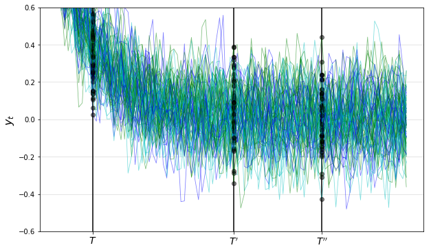
Note how the time series “settle down” in the sense that the distributions at \(T'\) and \(T''\) are relatively similar to each other — but unlike the distribution at \(T\).

Apparently, the distributions of \(y_t\) converge to a fixed long-run distribution as \(t \to \infty\).

When such a distribution exists it is called a stationary distribution.

24.4.2. Stationary Distributions#

In our setting, a distribution \(\psi_{\infty}\) is said to be stationary for \(x_t\) if

\[ x_t \sim \psi_{\infty} \quad \text{and} \quad x_{t+1} = A x_t + C w_{t+1} \quad \implies \quad x_{t+1} \sim \psi_{\infty} \]

Since

in the present case all distributions are Gaussian
a Gaussian distribution is pinned down by its mean and variance-covariance matrix

we can restate the definition as follows: \(\psi_{\infty}\) is stationary for \(x_t\) if

\[ \psi_{\infty} = N(\mu_{\infty}, \Sigma_{\infty}) \]

where \(\mu_{\infty}\) and \(\Sigma_{\infty}\) are fixed points of (24.6) and (24.7) respectively.

24.4.3. Covariance Stationary Processes#

Let’s see what happens to the preceding figure if we start \(x_0\) at the stationary distribution.

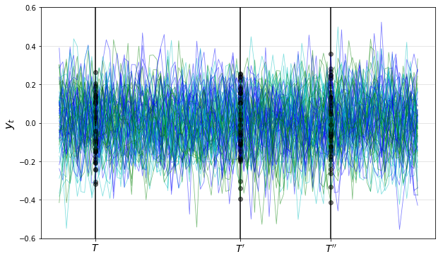
Now the differences in the observed distributions at \(T, T'\) and \(T''\) come entirely from random fluctuations due to the finite sample size.

our choosing \(x_0 \sim N(\mu_{\infty}, \Sigma_{\infty})\)
the definitions of \(\mu_{\infty}\) and \(\Sigma_{\infty}\) as fixed points of (24.6) and (24.7) respectively

we’ve ensured that

\[ \mu_t = \mu_{\infty} \quad \text{and} \quad \Sigma_t = \Sigma_{\infty} \quad \text{for all } t \]

Moreover, in view of (24.14), the autocovariance function takes the form \(\Sigma_{t+j,t} = A^j \Sigma_\infty\), which depends on \(j\) but not on \(t\).

This motivates the following definition.

A process \(\{x_t\}\) is said to be covariance stationary if

both \(\mu_t\) and \(\Sigma_t\) are constant in \(t\)
\(\Sigma_{t+j,t}\) depends on the time gap \(j\) but not on time \(t\)

In our setting, \(\{x_t\}\) will be covariance stationary if \(\mu_0, \Sigma_0, A, C\) assume values that imply that none of \(\mu_t, \Sigma_t, \Sigma_{t+j,t}\) depends on \(t\).

24.4.4. Conditions for Stationarity#

24.4.4.1. The globally stable case#

The difference equation \(\mu_{t+1} = A \mu_t\) is known to have unique fixed point \(\mu_{\infty} = 0\) if all eigenvalues of \(A\) have moduli strictly less than unity.

That is, if all(abs(eigvals(A)) .< 1) == true.

The difference equation (24.7) also has a unique fixed point in this case, and, moreover

\[ \mu_t \to \mu_{\infty} = 0 \quad \text{and} \quad \Sigma_t \to \Sigma_{\infty} \quad \text{as} \quad t \to \infty \]

regardless of the initial conditions \(\mu_0\) and \(\Sigma_0\).

This is the globally stable case — see these notes for more a theoretical treatment

However, global stability is more than we need for stationary solutions, and often more than we want.

To illustrate, consider our second order difference equation example.

Here the state is \(x_t = \begin{bmatrix} 1 & y_t & y_{t-1} \end{bmatrix}'\).

Because of the constant first component in the state vector, we will never have \(\mu_t \to 0\).

How can we find stationary solutions that respect a constant state component?

24.4.4.2. Processes with a constant state component#

To investigate such a process, suppose that \(A\) and \(C\) take the form

\[\begin{split} A = \begin{bmatrix} A_1 & a \\ 0 & 1 \end{bmatrix} \qquad C = \begin{bmatrix} C_1 \\ 0 \end{bmatrix} \end{split}\]

where

\(A_1\) is an \((n-1) \times (n-1)\) matrix
\(a\) is an \((n-1) \times 1\) column vector

Let \(x_t = \begin{bmatrix} x_{1t}' & 1 \end{bmatrix}'\) where \(x_{1t}\) is \((n-1) \times 1\).

It follows that

\[\begin{split} \begin{aligned} x_{1,t+1} & = A_1 x_{1t} + a + C_1 w_{t+1} \\ \end{aligned} \end{split}\]

Let \(\mu_{1t} = \mathbb{E} [x_{1t}]\) and take expectations on both sides of this expression to get

(24.15)#\[\mu_{1,t+1} = A_1 \mu_{1,t} + a\]

Assume now that the moduli of the eigenvalues of \(A_1\) are all strictly less than one.

Then (24.15) has a unique stationary solution, namely,

\[ \mu_{1\infty} = (I-A_1)^{-1} a \]

The stationary value of \(\mu_t\) itself is then \(\mu_\infty := \begin{bmatrix} \mu_{1\infty}' & 1 \end{bmatrix}'\).

The stationary values of \(\Sigma_t\) and \(\Sigma_{t+j,t}\) satisfy

(24.16)#\[\begin{split}\begin{aligned} \Sigma_\infty & = A \Sigma_\infty A' + C C' \\ \Sigma_{t+j,t} & = A^j \Sigma_\infty \nonumber \end{aligned}\end{split}\]

Notice that here \(\Sigma_{t+j,t}\) depends on the time gap \(j\) but not on calendar time \(t\).

In conclusion, if

\(x_0 \sim N(\mu_{\infty}, \Sigma_{\infty})\) and
the moduli of the eigenvalues of \(A_1\) are all strictly less than unity

then the \(\{x_t\}\) process is covariance stationary, with constant state component

Note

If the eigenvalues of \(A_1\) are less than unity in modulus, then (a) starting from any initial value, the mean and variance-covariance matrix both converge to their stationary values; and (b) iterations on (24.7) converge to the fixed point of the discrete Lyapunov equation in the first line of (24.16).

24.4.5. Ergodicity#

Let’s suppose that we’re working with a covariance stationary process.

In this case we know that the ensemble mean will converge to \(\mu_{\infty}\) as the sample size \(I\) approaches infinity.

24.4.5.1. Averages over time#

Ensemble averages across simulations are interesting theoretically, but in real life we usually observe only a single realization \(\{x_t, y_t\}_{t=0}^T\).

So now let’s take a single realization and form the time series averages

\[ \bar x := \frac{1}{T} \sum_{t=1}^T x_t \quad \text{and} \quad \bar y := \frac{1}{T} \sum_{t=1}^T y_t \]

Do these time series averages converge to something interpretable in terms of our basic state-space representation?

The answer depends on something called ergodicity.

Ergodicity is the property that time series and ensemble averages coincide.

More formally, ergodicity implies that time series sample averages converge to their expectation under the stationary distribution.

In particular,

\(\frac{1}{T} \sum_{t=1}^T x_t \to \mu_{\infty}\)
\(\frac{1}{T} \sum_{t=1}^T (x_t -\bar x_T) (x_t - \bar x_T)' \to \Sigma_\infty\)
\(\frac{1}{T} \sum_{t=1}^T (x_{t+j} -\bar x_T) (x_t - \bar x_T)' \to A^j \Sigma_\infty\)

In our linear Gaussian setting, any covariance stationary process is also ergodic.

24.5. Noisy Observations #

In some settings the observation equation \(y_t = Gx_t\) is modified to include an error term.

Often this error term represents the idea that the true state can only be observed imperfectly.

To include an error term in the observation we introduce

An iid sequence of \(\ell \times 1\) random vectors \(v_t \sim N(0,I)\)
A \(k \times \ell\) matrix \(H\)

and extend the linear state-space system to

(24.17)#\[\begin{split}\begin{aligned} x_{t+1} & = A x_t + C w_{t+1} \\ y_t & = G x_t + H v_t \nonumber \\ x_0 & \sim N(\mu_0, \Sigma_0) \nonumber \end{aligned}\end{split}\]

The sequence \(\{v_t\}\) is assumed to be independent of \(\{w_t\}\).

The process \(\{x_t\}\) is not modified by noise in the observation equation and its moments, distributions and stability properties remain the same.

The unconditional moments of \(y_t\) from (24.8) and (24.9) now become

(24.18)#\[\mathbb{E} [y_t] = \mathbb{E} [G x_t + H v_t] = G \mu_t\]

The variance-covariance matrix of \(y_t\) is easily shown to be

(24.19)#\[\textrm{Var} [y_t] = \textrm{Var} [G x_t + H v_t] = G \Sigma_t G' + HH'\]

The distribution of \(y_t\) is therefore

\[ y_t \sim N(G \mu_t, G \Sigma_t G' + HH') \]

24.6. Prediction #

The theory of prediction for linear state space systems is elegant and simple.

24.6.1. Forecasting Formulas – Conditional Means#

The natural way to predict variables is to use conditional distributions.

For example, the optimal forecast of \(x_{t+1}\) given information known at time \(t\) is

\[ \mathbb{E}_t [x_{t+1}] := \mathbb{E} [x_{t+1} \mid x_t, x_{t-1}, \ldots, x_0 ] = Ax_t \]

The right-hand side follows from \(x_{t+1} = A x_t + C w_{t+1}\) and the fact that \(w_{t+1}\) is zero mean and independent of \(x_t, x_{t-1}, \ldots, x_0\).

That \(\mathbb{E}_t [x_{t+1}] = \mathbb{E}[x_{t+1} \mid x_t]\) is an implication of \(\{x_t\}\) having the Markov property.

The one-step-ahead forecast error is

\[ x_{t+1} - \mathbb{E}_t [x_{t+1}] = Cw_{t+1} \]

The covariance matrix of the forecast error is

\[ \mathbb{E} [ (x_{t+1} - \mathbb{E}_t [ x_{t+1}] ) (x_{t+1} - \mathbb{E}_t [ x_{t+1}])'] = CC' \]

More generally, we’d like to compute the \(j\)-step ahead forecasts \(\mathbb{E}_t [x_{t+j}]\) and \(\mathbb{E}_t [y_{t+j}]\).

With a bit of algebra we obtain

\[ x_{t+j} = A^j x_t + A^{j-1} C w_{t+1} + A^{j-2} C w_{t+2} + \cdots + A^0 C w_{t+j} \]

In view of the iid property, current and past state values provide no information about future values of the shock.

Hence \(\mathbb{E}_t[w_{t+k}] = \mathbb{E}[w_{t+k}] = 0\).

It now follows from linearity of expectations that the \(j\)-step ahead forecast of \(x\) is

\[ \mathbb{E}_t [x_{t+j}] = A^j x_t \]

The \(j\)-step ahead forecast of \(y\) is therefore

\[ \mathbb{E}_t [y_{t+j}] = \mathbb{E}_t [G x_{t+j} + H v_{t+j}] = G A^j x_t \]

24.6.2. Covariance of Prediction Errors#

It is useful to obtain the covariance matrix of the vector of \(j\)-step-ahead prediction errors

(24.20)#\[x_{t+j} - \mathbb{E}_t [ x_{t+j}] = \sum^{j-1}_{s=0} A^s C w_{t-s+j}\]

Evidently,

(24.21)#\[V_j := \mathbb{E}_t [ (x_{t+j} - \mathbb{E}_t [x_{t+j}] ) (x_{t+j} - \mathbb{E}_t [x_{t+j}] )^\prime ] = \sum^{j-1}_{k=0} A^k C C^\prime A^{k^\prime}\]

\(V_j\) defined in (24.21) can be calculated recursively via \(V_1 = CC'\) and

(24.22)#\[V_j = CC^\prime + A V_{j-1} A^\prime, \quad j \geq 2\]

\(V_j\) is the conditional covariance matrix of the errors in forecasting \(x_{t+j}\), conditioned on time \(t\) information \(x_t\).

Under particular conditions, \(V_j\) converges to

(24.23)#\[V_\infty = CC' + A V_\infty A'\]

Equation (24.23) is an example of a discrete Lyapunov equation in the covariance matrix \(V_\infty\).

A sufficient condition for \(V_j\) to converge is that the eigenvalues of \(A\) be strictly less than one in modulus.

Weaker sufficient conditions for convergence associate eigenvalues equaling or exceeding one in modulus with elements of \(C\) that equal \(0\).

24.6.3. Forecasts of Geometric Sums#

In several contexts, we want to compute forecasts of geometric sums of future random variables governed by the linear state-space system (24.1).

We want the following objects

Forecast of a geometric sum of future \(x\)’s, or \(\mathbb{E}_t \left[ \sum_{j=0}^\infty \beta^j x_{t+j} \right]\).
Forecast of a geometric sum of future \(y\)’s, or \(\mathbb{E}_t \left[\sum_{j=0}^\infty \beta^j y_{t+j} \right]\).

These objects are important components of some famous and interesting dynamic models.

For example,

if \(\{y_t\}\) is a stream of dividends, then \(\mathbb{E} \left[\sum_{j=0}^\infty \beta^j y_{t+j} | x_t \right]\) is a model of a stock price
if \(\{y_t\}\) is the money supply, then \(\mathbb{E} \left[\sum_{j=0}^\infty \beta^j y_{t+j} | x_t \right]\) is a model of the price level

24.6.3.1. Formulas#

Fortunately, it is easy to use a little matrix algebra to compute these objects.

Suppose that every eigenvalue of \(A\) has modulus strictly less than \(\frac{1}{\beta}\).

It then follows that \(I + \beta A + \beta^2 A^2 + \cdots = \left[I - \beta A \right]^{-1}\).

This leads to our formulas:

Forecast of a geometric sum of future \(x\)’s

\[ \mathbb{E}_t \left[\sum_{j=0}^\infty \beta^j x_{t+j} \right] = [I + \beta A + \beta^2 A^2 + \cdots \ ] x_t = [I - \beta A]^{-1} x_t \]

Forecast of a geometric sum of future \(y\)’s

\[ \mathbb{E}_t \left[\sum_{j=0}^\infty \beta^j y_{t+j} \right] = G [I + \beta A + \beta^2 A^2 + \cdots \ ] x_t = G[I - \beta A]^{-1} x_t \]

24.7. Code #

Our preceding simulations and calculations are based on code in the file lss.jl from the QuantEcon.jl package.

The code implements a type which the linear state space models can act on directly through specific methods (for simulations, calculating moments, etc.).

Examples of usage are given in the solutions to the exercises.

24.8. Exercises #

24.8.1. Exercise 1#

Replicate this figure using the LSS type from lss.jl.

24.8.2. Exercise 2#

Replicate this figure modulo randomness using the same type.

24.8.3. Exercise 3#

Replicate this figure modulo randomness using the same type.

The state space model and parameters are the same as for the preceding exercise.

24.8.4. Exercise 4#

Replicate this figure modulo randomness using the same type.

The state space model and parameters are the same as for the preceding exercise, except that the initial condition is the stationary distribution.

Hint: You can use the stationary_distributions method to get the initial conditions.

The number of sample paths is 80, and the time horizon in the figure is 100.

Producing the vertical bars and dots is optional, but if you wish to try, the bars are at dates 10, 50 and 75.

24.9. Solutions #

using LaTeXStrings, QuantEcon, Plots

24.9.1. Exercise 1#

phi0, phi1, phi2 = 1.1, 0.8, -0.8

A = [1.0 0.0 0
     phi0 phi1 phi2
     0.0 1.0 0.0]
C = zeros(3, 1)
G = [0.0 1.0 0.0]
mu_0 = ones(3)

lss = LSS(A, C, G; mu_0)

x, y = simulate(lss, 50)
plot(dropdims(y, dims = 1), color = :blue, linewidth = 2, alpha = 0.7)
plot!(xlabel = "time", ylabel = L"y_t", legend = :none)

24.9.2. Exercise 2#

using Random
Random.seed!(42) # For deterministic results.

phi1, phi2, phi3, phi4 = 0.5, -0.2, 0, 0.5
sigma = 0.2

A = [phi1 phi2 phi3 phi4
     1.0 0.0 0.0 0.0
     0.0 1.0 0.0 0.0
     0.0 0.0 1.0 0.0]
C = [sigma
     0.0
     0.0
     0.0]
G = [1.0 0.0 0.0 0.0]

ar = LSS(A, C, G; mu_0 = ones(4))
x, y = simulate(ar, 200)

plot(dropdims(y, dims = 1), color = :blue, linewidth = 2, alpha = 0.7)
plot!(xlabel = "time", ylabel = L"y_t", legend = :none)

24.9.3. Exercise 3#

phi1, phi2, phi3, phi4 = 0.5, -0.2, 0, 0.5
sigma = 0.1

A = [phi1 phi2 phi3 phi4
     1.0 0.0 0.0 0.0
     0.0 1.0 0.0 0.0
     0.0 0.0 1.0 0.0]
C = [sigma
     0.0
     0.0
     0.0]
G = [1.0 0.0 0.0 0.0]
I = 20
T = 50
ar = LSS(A, C, G; mu_0 = ones(4))
ymin, ymax = -0.5, 1.15

ensemble_mean = zeros(T)
ys = []
for i in 1:I
    x, y = simulate(ar, T)
    y = dropdims(y, dims = 1)
    push!(ys, y)
    ensemble_mean .+= y
end

ensemble_mean = ensemble_mean ./ I
plot(ys, color = :blue, alpha = 0.2, linewidth = 0.8, label = "")
plot!(ensemble_mean, color = :blue, linewidth = 2, label = L"\overline{y_t}")
m = moment_sequence(ar)
pop_means = zeros(0)
for (i, t) in enumerate(m)
    (mu_x, mu_y, Sigma_x, Sigma_y) = t
    push!(pop_means, mu_y[1])
    i == 50 && break
end
plot!(pop_means, color = :green, linewidth = 2, label = L"G \mu_t")
plot!(ylims = (ymin, ymax), xlabel = "time", ylabel = L"y_t", legendfont = font(12))

24.9.4. Exercise 4#

phi1, phi2, phi3, phi4 = 0.5, -0.2, 0, 0.5
sigma = 0.1

A = [phi1 phi2 phi3 phi4
     1.0 0.0 0.0 0.0
     0.0 1.0 0.0 0.0
     0.0 0.0 1.0 0.0]
C = [sigma
     0.0
     0.0
     0.0]
G = [1.0 0.0 0.0 0.0]

T0 = 10
T1 = 50
T2 = 75
T4 = 100

ar = LSS(A, C, G; mu_0 = ones(4))
ymin, ymax = -0.6, 0.6

mu_x, mu_y, Sigma_x, Sigma_y = stationary_distributions(ar)
ar = LSS(A, C, G; mu_0 = mu_x, Sigma_0 = Sigma_x)
colors = ["c", "g", "b"]

ys = []
x_scatter = []
y_scatter = []
for i in 1:80
    rcolor = colors[rand(1:3)]
    x, y = simulate(ar, T4)
    y = dropdims(y, dims = 1)
    push!(ys, y)
    x_scatter = [x_scatter; T0; T1; T2]
    y_scatter = [y_scatter; y[T0]; y[T1]; y[T2]]
end

plot(ys, linewidth = 0.8, alpha = 0.5)
plot!([T0 T1 T2; T0 T1 T2], [-1 -1 -1; 1 1 1], color = :black, legend = :none)
scatter!(x_scatter, y_scatter, color = :black, alpha = 0.5)
plot!(ylims = (ymin, ymax), ylabel = L"y_t", xticks = [], yticks = ymin:0.2:ymax)
plot!(annotations = [(T0 + 1, -0.55, L"T"); (T1 + 1, -0.55, L"T^\prime");
                     (T2 + 1, -0.55, L"T^{\prime\prime}")])

1: The eigenvalues of \(A\) are \((1,-1, i,-i)\).
2: The correct way to argue this is by induction. Suppose that \(x_t\) is Gaussian. Then (24.1) and (24.10) imply that \(x_{t+1}\) is Gaussian. Since \(x_0\) is assumed to be Gaussian, it follows that every \(x_t\) is Gaussian. Evidently this implies that each \(y_t\) is Gaussian.