51. A Lake Model of Employment and Unemployment#
Contents
51.1. Overview#
This lecture describes what has come to be called a lake model.
The lake model is a basic tool for modeling unemployment.
It allows us to analyze
flows between unemployment and employment
how these flows influence steady state employment and unemployment rates
It is a good model for interpreting monthly labor department reports on gross and net jobs created and jobs destroyed.
The “lakes” in the model are the pools of employed and unemployed.
The “flows” between the lakes are caused by
firing and hiring
entry and exit from the labor force
For the first part of this lecture, the parameters governing transitions into and out of unemployment and employment are exogenous.
Later, we’ll determine some of these transition rates endogenously using the McCall search model.
We’ll also use some nifty concepts like ergodicity, which provides a fundamental link between cross-sectional and long run time series distributions.
These concepts will help us build an equilibrium model of ex ante homogeneous workers whose different luck generates variations in their ex post experiences.
51.1.1. Prerequisites#
Before working through what follows, we recommend you read the lecture on finite Markov chains.
You will also need some basic linear algebra and probability.
51.2. The Model#
The economy is inhabited by a very large number of ex ante identical workers.
The workers live forever, spending their lives moving between unemployment and employment.
Their rates of transition between employment and unemployment are governed by the following parameters:
\(\lambda\), the job finding rate for currently unemployed workers
\(\alpha\), the dismissal rate for currently employed workers
\(b\), the entry rate into the labor force
\(d\), the exit rate from the labor force
The growth rate of the labor force evidently equals \(g=b-d\).
51.2.1. Aggregate Variables#
We want to derive the dynamics of the following aggregates
\(E_t\), the total number of employed workers at date \(t\)
\(U_t\), the total number of unemployed workers at \(t\)
\(N_t\), the number of workers in the labor force at \(t\)
We also want to know the values of the following objects
The employment rate \(e_t := E_t/N_t\).
The unemployment rate \(u_t := U_t/N_t\).
(Here and below, capital letters represent stocks and lowercase letters represent flows)
51.2.2. Laws of Motion for Stock Variables#
We begin by constructing laws of motion for the aggregate variables \(E_t,U_t, N_t\).
Of the mass of workers \(E_t\) who are employed at date \(t\),
\((1-d)E_t\) will remain in the labor force
of these, \((1-\alpha)(1-d)E_t\) will remain employed
Of the mass of workers \(U_t\) workers who are currently unemployed,
\((1-d)U_t\) will remain in the labor force
of these, \((1-d) \lambda U_t\) will become employed
Therefore, the number of workers who will be employed at date \(t+1\) will be
A similar analysis implies
The value \(b(E_t+U_t)\) is the mass of new workers entering the labor force unemployed.
The total stock of workers \(N_t=E_t+U_t\) evolves as
Letting \(X_t := \left(\begin{matrix}U_t\\E_t\end{matrix}\right)\), the law of motion for \(X\) is
This law tells us how total employment and unemployment evolve over time.
51.2.3. Laws of Motion for Rates#
Now let’s derive the law of motion for rates.
To get these we can divide both sides of \(X_{t+1} = A X_t\) by \(N_{t+1}\) to get
Letting
we can also write this as
You can check that \(e_t + u_t = 1\) implies that \(e_{t+1}+u_{t+1} = 1\).
This follows from the fact that the columns of \(\hat A\) sum to 1.
51.3. Implementation#
Let’s code up these equations.
Here’s the code:
using Pkg; pkgs = ["Distributions", "NLsolve", "Plots", "Roots"]; all(haskey.(Ref(Pkg.project().dependencies), pkgs)) || Pkg.add(pkgs)
using LinearAlgebra, Statistics, Distributions
using NLsolve, Roots, Random
using Plots
Reusable functions for simulating linear maps and finding their fixed points
function simulate_linear(A, x_0, T)
    X = zeros(length(x_0), T + 1)
    X[:, 1] = x_0
    for t in 2:(T + 1)
        X[:, t] = A * X[:, t - 1]
    end
    return X
end

function linear_steady_state(A, x_0 = ones(size(A, 1)) / size(A, 1))
    sol = fixedpoint(x -> A * x, x_0)
    converged(sol) || error("Failed to converge in $(sol.iterations) iter")
    return sol.zero
end
linear_steady_state (generic function with 2 methods)
function lake_model(; lambda = 0.283, alpha = 0.013, b = 0.0124, d = 0.00822)
    # calculate transition matrices
    g = b - d
    A = [(1 - lambda) * (1 - d)+b (1 - d) * alpha+b
         (1 - d)*lambda (1 - d)*(1 - alpha)]
    A_hat = A ./ (1 + g)

    # Solve for fixed point to find the steady-state u and e
    x_bar = linear_steady_state(A_hat)
    return (; lambda, alpha, b, d, A, A_hat, x_bar)
end
lake_model (generic function with 1 method)
Let’s observe these matrices for the baseline model
lm = lake_model()
lm.A
2×2 Matrix{Float64}:
 0.723506  0.0252931
 0.280674  0.978887
lm.A_hat
2×2 Matrix{Float64}:
 0.720495  0.0251879
 0.279505  0.974812
And a revised model
lm = lake_model(; alpha = 0.2)
lm.A
2×2 Matrix{Float64}:
 0.723506  0.210756
 0.280674  0.793424
lm.A_hat
2×2 Matrix{Float64}:
 0.720495  0.209879
 0.279505  0.790121
51.3.1. Aggregate Dynamics#
Let’s run a simulation under the default parameters (see above) starting from \(X_0 = (12, 138)\)
lm = lake_model()
N_0 = 150      # population
e_0 = 0.92     # initial employment rate
u_0 = 1 - e_0  # initial unemployment rate
T = 50         # simulation length

U_0 = u_0 * N_0
E_0 = e_0 * N_0
X_0 = [U_0; E_0]

X_path = simulate_linear(lm.A, X_0, T - 1)

x1 = X_path[1, :]
x2 = X_path[2, :]
x3 = sum(X_path, dims = 1)'

plt_unemp = plot(title = "Unemployment", 1:T, x1, color = :blue, lw = 2,
                 grid = true, label = "")
plt_emp = plot(title = "Employment", 1:T, x2, color = :blue, lw = 2,
               grid = true, label = "")
plt_labor = plot(title = "Labor force", 1:T, x3, color = :blue, lw = 2,
                 grid = true, label = "")

plot(plt_unemp, plt_emp, plt_labor, layout = (3, 1), size = (800, 600))

The aggregates \(E_t\) and \(U_t\) don’t converge because their sum \(E_t + U_t\) grows at rate \(g\).
On the other hand, the vector of employment and unemployment rates \(x_t\) can be in a steady state \(\bar x\) if there exists an \(\bar x\) such that
\(\bar x = \hat A \bar x\)
the components satisfy \(\bar e + \bar u = 1\)
This equation tells us that a steady state level \(\bar x\) is an eigenvector of \(\hat A\) associated with a unit eigenvalue.
We also have \(x_t \to \bar x\) as \(t \to \infty\) provided that the remaining eigenvalue of \(\hat A\) has modulus less that 1.
This is the case for our default parameters:
lm = lake_model()
e, f = eigvals(lm.A_hat)
abs(e), abs(f)
(0.6953067378358462, 1.0)
Let’s look at the convergence of the unemployment and employment rate to steady state levels (dashed red line)
lm = lake_model()
e_0 = 0.92 # initial employment rate
u_0 = 1 - e_0 # initial unemployment rate
T = 50 # simulation length

u_bar, e_bar = lm.x_bar
x_0 = [u_0; e_0]
x_path = simulate_linear(lm.A_hat, x_0, T - 1)

plt_unemp = plot(title = "Unemployment rate", 1:T, x_path[1, :], color = :blue,
                 lw = 2, alpha = 0.5, grid = true, label = "")
plot!(plt_unemp, [u_bar], color = :red, linetype = :hline, linestyle = :dash,
      lw = 2, label = "")
plt_emp = plot(title = "Employment rate", 1:T, x_path[2, :], color = :blue,
               lw = 2, alpha = 0.5, grid = true, label = "")
plot!(plt_emp, [e_bar], color = :red, linetype = :hline, linestyle = :dash,
      lw = 2, label = "")
plot(plt_unemp, plt_emp, layout = (2, 1), size = (700, 500))

51.4. Dynamics of an Individual Worker#
An individual worker’s employment dynamics are governed by a finite state Markov process.
The worker can be in one of two states:
\(s_t=0\) means unemployed
\(s_t=1\) means employed
Let’s start off under the assumption that \(b = d = 0\).
The associated transition matrix is then
Let \(\psi_t\) denote the marginal distribution over employment / unemployment states for the worker at time \(t\).
As usual, we regard it as a row vector.
We know from an earlier discussion that \(\psi_t\) follows the law of motion
We also know from the lecture on finite Markov chains that if \(\alpha \in (0, 1)\) and \(\lambda \in (0, 1)\), then \(P\) has a unique stationary distribution, denoted here by \(\psi^*\).
The unique stationary distribution satisfies
Not surprisingly, probability mass on the unemployment state increases with the dismissal rate and falls with the job finding rate rate.
51.4.1. Ergodicity#
Let’s look at a typical lifetime of employment-unemployment spells.
We want to compute the average amounts of time an infinitely lived worker would spend employed and unemployed.
Let
and
(As usual, \(\mathbb 1\{Q\} = 1\) if statement \(Q\) is true and 0 otherwise)
These are the fraction of time a worker spends unemployed and employed, respectively, up until period \(T\).
If \(\alpha \in (0, 1)\) and \(\lambda \in (0, 1)\), then \(P\) is ergodic, and hence we have
with probability one.
Inspection tells us that \(P\) is exactly the transpose of \(\hat A\) under the assumption \(b=d=0\).
Thus, the percentages of time that an infinitely lived worker spends employed and unemployed equal the fractions of workers employed and unemployed in the steady state distribution.
51.4.2. Convergence rate#
How long does it take for time series sample averages to converge to cross sectional averages?
We can use a simple simulator to generate sample paths.
function simulate_markov_chain(P, X_0, T)
    N = size(P, 1)
    num_chains = length(X_0)
    P_dist = [Categorical(P[i, :]) for i in 1:N]
    X = zeros(Int, num_chains, T + 1)
    X[:, 1] .= X_0
    for t in 1:T
        for n in 1:num_chains
            X[n, t+1] = rand(P_dist[X[n, t]])
        end
    end
    return X
end
simulate_markov_chain (generic function with 1 method)
Let’s plot the path of the sample averages over 5,000 periods
lm = lake_model(; d = 0, b = 0)
T = 5000                        # Simulation length

(; alpha, lambda) = lm
P = [(1-lambda) lambda
     alpha (1-alpha)]
2×2 Matrix{Float64}:
 0.717  0.283
 0.013  0.987
Random.seed!(42)
u_bar, e_bar = lm.x_bar
X = simulate_markov_chain(P, [2], T)
states = [0, 1]
s_path = states[X[1, 2:end]]  # map indices to 0/1 labels

s_bar_e = cumsum(s_path) ./ (1:T)
s_bar_u = 1 .- s_bar_e
s_bars = [s_bar_u s_bar_e]

plt_unemp = plot(title = "Percent of time unemployed", 1:T, s_bars[:, 1],
                 color = :blue, lw = 2, alpha = 0.5, label = "", grid = true)
plot!(plt_unemp, [u_bar], linetype = :hline, linestyle = :dash, color = :red,
      lw = 2, label = "")
plt_emp = plot(title = "Percent of time employed", 1:T, s_bars[:, 2],
               color = :blue, lw = 2, alpha = 0.5, label = "", grid = true)
plot!(plt_emp, [e_bar], linetype = :hline, linestyle = :dash, color = :red,
      lw = 2, label = "")
plot(plt_unemp, plt_emp, layout = (2, 1), size = (700, 500))

The stationary probabilities are given by the dashed red line.
In this case it takes much of the sample for these two objects to converge.
This is largely due to the high persistence in the Markov chain.
51.5. Endogenous Job Finding Rate#
We now make the hiring rate endogenous.
The transition rate from unemployment to employment will be determined by the McCall search model [McC70].
All details relevant to the following discussion can be found in our treatment of that model.
51.5.1. Reservation Wage#
The most important thing to remember about the model is that optimal decisions are characterized by a reservation wage \(\bar w\).
If the wage offer \(w\) in hand is greater than or equal to \(\bar w\), then the worker accepts.
Otherwise, the worker rejects.
As we saw in our discussion of the model, the reservation wage depends on the wage offer distribution and the parameters
\(\alpha\), the separation rate
\(\beta\), the discount factor
\(\gamma\), the offer arrival rate
\(c\), unemployment compensation
51.5.2. Linking the McCall Search Model to the Lake Model#
Suppose that all workers inside a lake model behave according to the McCall search model.
The exogenous probability of leaving employment remains \(\alpha\).
But their optimal decision rules determine the probability \(\lambda\) of leaving unemployment.
This is now
51.5.3. Fiscal Policy#
We can use the McCall search version of the Lake Model to find an optimal level of unemployment insurance.
We assume that the government sets unemployment compensation \(c\).
The government imposes a lump sum tax \(\tau\) sufficient to finance total unemployment payments.
To attain a balanced budget at a steady state, taxes, the steady state unemployment rate \(u\), and the unemployment compensation rate must satisfy
The lump sum tax applies to everyone, including unemployed workers.
Thus, the post-tax income of an employed worker with wage \(w\) is \(w - \tau\).
The post-tax income of an unemployed worker is \(c - \tau\).
For each specification \((c, \tau)\) of government policy, we can solve for the worker’s optimal reservation wage.
This determines \(\lambda\) via (51.1) evaluated at post tax wages, which in turn determines a steady state unemployment rate \(u(c, \tau)\).
For a given level of unemployment benefit \(c\), we can solve for a tax that balances the budget in the steady state
To evaluate alternative government tax-unemployment compensation pairs, we require a welfare criterion.
We use a steady state welfare criterion
where the notation \(V\) and \(U\) is as defined in the McCall search model lecture.
The wage offer distribution will be a discretized version of the lognormal distribution \(LN(\log(20),1)\), as shown in the next figure
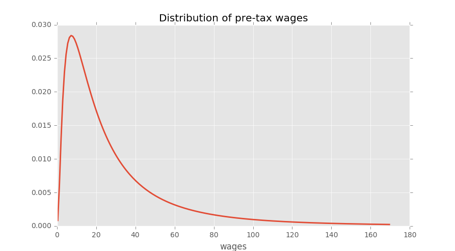
We take a period to be a month.
We set \(b\) and \(d\) to match monthly birth and death rates, respectively, in the U.S. population
\(b = 0.0124\)
\(d = 0.00822\)
Following [DFH06], we set \(\alpha\), the hazard rate of leaving employment, to
\(\alpha = 0.013\)
51.5.4. Fiscal Policy Code#
We will make use of (with some tweaks) the code we wrote in the McCall model lecture, embedded below for convenience.
function solve_mccall_model(mcm; U_iv = 1.0, V_iv = ones(length(mcm.w)),
                            tol = 1e-5, iter = 2_000)
    (; alpha, beta, sigma, c, gamma, w, u, w_probs) = mcm

    @assert c > 0.0
    u_w = mcm.u.(w)
    u_c = mcm.u(c)
    # Bellman operator T. Fixed point is x* s.t. T(x*) = x*
    function T(x)
        V = x[1:(end - 1)]
        U = x[end]
        V_p = u_w + beta * ((1 - alpha) * V .+ alpha * U)
        U_p = u_c + beta * (1 - gamma) * U +
              beta * gamma * sum(max(U, V[i]) * w_probs[i] for i in 1:length(w))
        # return [u_w + beta * ((1 - alpha) * V .+ alpha * U); u_c + beta * (1 - gamma) * U + beta * gamma * dot(w_probs, max.(U, V))]
        return [V_p; U_p]
    end

    # value function iteration
    x_iv = [V_iv; U_iv] # initial x val
    xstar = fixedpoint(T, x_iv, iterations = iter, xtol = tol, m = 0).zero
    V = xstar[1:(end - 1)]
    U = xstar[end]

    # compute the reservation wage
    w_bar_index = searchsortedfirst(V .- U, 0.0)
    if w_bar_index >= length(w) # if this is true, you never want to accept
        w_bar = Inf
    else
        w_bar = w[w_bar_index] # otherwise, return the number
    end

    # return a NamedTuple, so we can select values by name
    return (; V, U, w_bar)
end
solve_mccall_model (generic function with 1 method)
And the McCall object
u_crra(c, sigma) = c > 0 ? (c^(1 - sigma) - 1) / (1 - sigma) : -10e-6

function mccall_model(; alpha, beta, gamma, c, sigma, w, w_probs,
                      u = c -> u_crra(c, sigma))
    return (; alpha, beta, gamma, c, sigma, u, w, w_probs)
end
mccall_model (generic function with 1 method)
Now let’s compute and plot welfare, employment, unemployment, and tax revenue as a function of the unemployment compensation rate
function compute_optimal_quantities(c_pretax, tau; w_probs, sigma, gamma, beta,
                                    alpha, w_pretax)
    mcm = mccall_model(; alpha, beta, gamma, sigma, w_probs, c = c_pretax - tau,
                       w = w_pretax .- tau)
    w_probs = mcm.w_probs
    (; V, U, w_bar) = solve_mccall_model(mcm)
    accept_wage = w_pretax .- tau .> w_bar

    # sum up proportion accepting the wages
    lambda = gamma * dot(w_probs, accept_wage)
    return w_bar, lambda, V, U, w_probs
end

function compute_steady_state_quantities(c_pretax, tau; w_probs, sigma, gamma,
                                         beta, alpha, w_pretax, b, d)
    w_bar, lambda, V, U,
    w_probs = compute_optimal_quantities(c_pretax, tau; w_probs, sigma, gamma,
                                         beta, alpha, w_pretax)

    # compute steady state employment and unemployment rates
    lm = lake_model(; lambda, alpha, b, d)
    u_rate, e_rate = lm.x_bar

    # compute steady state welfare
    accept_wage = w_pretax .- tau .> w_bar
    w = (dot(w_probs, V .* accept_wage)) / dot(w_probs, accept_wage)
    welfare = e_rate .* w + u_rate .* U

    return u_rate, e_rate, welfare
end

function find_balanced_budget_tax(c_pretax; w_probs, sigma, gamma, beta, alpha,
                                  w_pretax, b, d)
    function steady_state_budget(t)
        u_rate, e_rate,
        w = compute_steady_state_quantities(c_pretax, t; w_probs, sigma, gamma,
                                            beta, alpha, w_pretax, b, d)
        return t - u_rate * c_pretax
    end

    tau = find_zero(steady_state_budget, (0.0, 0.9 * c_pretax))
    return tau
end
find_balanced_budget_tax (generic function with 1 method)
Helper function to calculate for various unemployment insurance levels
function calculate_equilibriums(c_pretax; w_probs, sigma, gamma, beta, alpha,
                                w_pretax, b, d)
    tau_vec = similar(c_pretax)
    u_vec = similar(c_pretax)
    e_vec = similar(c_pretax)
    welfare_vec = similar(c_pretax)

    for (i, c_pre) in enumerate(c_pretax)
        tau = find_balanced_budget_tax(c_pre; w_probs, sigma, gamma, beta,
                                       alpha, w_pretax, b, d)
        u_rate, e_rate,
        welfare = compute_steady_state_quantities(c_pre, tau; w_probs, sigma,
                                                  gamma, beta, alpha, w_pretax,
                                                  b, d)
        tau_vec[i] = tau
        u_vec[i] = u_rate
        e_vec[i] = e_rate
        welfare_vec[i] = welfare
    end
    return tau_vec, u_vec, e_vec, welfare_vec
end
calculate_equilibriums (generic function with 1 method)
Parameters for our experiment
alpha_base = 0.013
alpha = (1 - (1 - alpha_base)^3)
b = 0.0124
d = 0.00822
beta = 0.98
gamma = 1.0
sigma = 2.0

# the default wage distribution: a discretized log normal
log_wage_mean, wage_grid_size, max_wage = 20, 200, 170
w_pretax = range(1e-3, max_wage, length = wage_grid_size + 1)
logw_dist = Normal(log(log_wage_mean), 1)
cdf_logw = cdf.(logw_dist, log.(w_pretax))
pdf_logw = cdf_logw[2:end] - cdf_logw[1:(end - 1)]
w_probs = pdf_logw ./ sum(pdf_logw) # probabilities
w_pretax = (w_pretax[1:(end - 1)] + w_pretax[2:end]) / 2

# levels of unemployment insurance we wish to study
c_pretax = range(5, 140, length = 60)
tau_vec, u_vec, e_vec,
welfare_vec = calculate_equilibriums(c_pretax; w_probs, sigma, gamma, beta,
                                     alpha, w_pretax, b, d)

# plots
plt_unemp = plot(title = "Unemployment", c_pretax, u_vec, color = :blue,
                 lw = 2, alpha = 0.7, label = "", grid = true)
plt_tax = plot(title = "Tax", c_pretax, tau_vec, color = :blue, lw = 2,
               alpha = 0.7, label = "", grid = true)
plt_emp = plot(title = "Employment", c_pretax, e_vec, color = :blue, lw = 2,
               alpha = 0.7, label = "", grid = true)
plt_welf = plot(title = "Welfare", c_pretax, welfare_vec, color = :blue, lw = 2,
                alpha = 0.7, label = "", grid = true)

plot(plt_unemp, plt_emp, plt_tax, plt_welf, layout = (2, 2), size = (800, 700))

Welfare first increases and then decreases as unemployment benefits rise.
The level that maximizes steady state welfare is approximately 62.
51.6. Exercises#
51.6.1. Exercise 1#
Consider an economy with initial stock of workers \(N_0 = 100\) at the steady state level of employment in the baseline parameterization
\(\alpha = 0.013\)
\(\lambda = 0.283\)
\(b = 0.0124\)
\(d = 0.00822\)
(The values for \(\alpha\) and \(\lambda\) follow [DFH06])
Suppose that in response to new legislation the hiring rate reduces to \(\lambda = 0.2\).
Plot the transition dynamics of the unemployment and employment stocks for 50 periods.
Plot the transition dynamics for the rates.
How long does the economy take to converge to its new steady state?
What is the new steady state level of employment?
51.6.2. Exercise 2#
Consider an economy with initial stock of workers \(N_0 = 100\) at the steady state level of employment in the baseline parameterization.
Suppose that for 20 periods the birth rate was temporarily high (\(b = 0.0025\)) and then returned to its original level.
Plot the transition dynamics of the unemployment and employment stocks for 50 periods.
Plot the transition dynamics for the rates.
How long does the economy take to return to its original steady state?
51.7. Solutions#
51.7.1. Exercise 1#
We begin by constructing an object containing the default parameters and assigning the steady state values to x0
lm = lake_model()
x0 = lm.x_bar
println("Initial Steady State: $x0")
Initial Steady State: [0.08266626766923271, 0.9173337323307673]
Initialize the simulation values
N0 = 100
T = 50
50
New legislation changes \(\lambda\) to \(0.2\)
lm = lake_model(; lambda = 0.2)
X_path = simulate_linear(lm.A, x0 * N0, T - 1)
x_path = simulate_linear(lm.A_hat, x0, T - 1)
u_bar, e_bar = lm.x_bar
println("New Steady State: [$u_bar, $e_bar]")
New Steady State: [0.11309294549489424, 0.8869070545051054]
Now plot stocks
x1 = X_path[1, :]
x2 = X_path[2, :]
x3 = sum(X_path, dims = 1)'

plt_unemp = plot(title = "Unemployment", 1:T, x1, color = :blue, grid = true,
                 label = "", bg_inside = :lightgrey)
plt_emp = plot(title = "Employment", 1:T, x2, color = :blue, grid = true,
               label = "", bg_inside = :lightgrey)
plt_labor = plot(title = "Labor force", 1:T, x3, color = :blue, grid = true,
                 label = "", bg_inside = :lightgrey)

plot(plt_unemp, plt_emp, plt_labor, layout = (3, 1), size = (800, 600))

And how the rates evolve
plt_unemp = plot(title = "Unemployment rate", 1:T, x_path[1, :], color = :blue,
                 grid = true, label = "", bg_inside = :lightgrey)
plot!(plt_unemp, [u_bar], linetype = :hline, linestyle = :dash, color = :red,
      label = "")

plt_emp = plot(title = "Employment rate", 1:T, x_path[2, :], color = :blue,
               grid = true, label = "", bg_inside = :lightgrey)
plot!(plt_emp, [e_bar], linetype = :hline, linestyle = :dash, color = :red,
      label = "")
plot(plt_unemp, plt_emp, layout = (2, 1), size = (800, 600))

We see that it takes 20 periods for the economy to converge to it’s new steady state levels.
51.7.2. Exercise 2#
This next exercise has the economy experiencing a boom in entrances to the labor market and then later returning to the original levels.
For 20 periods the economy has a new entry rate into the labor market.
Let’s start off at the baseline parameterization and record the steady state
lm = lake_model()
x0 = lm.x_bar
2-element Vector{Float64}:
 0.08266626766923271
 0.9173337323307673
Here are the other parameters:
b_hat = 0.003
T_hat = 20
20
Let’s increase \(b\) to the new value and simulate for 20 periods
lm = lake_model(; b = b_hat)
X_path1 = simulate_linear(lm.A, x0 * N0, T_hat - 1)
x_path1 = simulate_linear(lm.A_hat, x0, T_hat - 1)
2×20 Matrix{Float64}:
 0.0826663  0.0739981  0.0679141  …  0.0536612  0.0536401  0.0536253
 0.917334   0.926002   0.932086      0.946339   0.94636    0.946375
Now we reset \(b\) to the original value and then, using the state after 20 periods for the new initial conditions, we simulate for the additional 30 periods
lm = lake_model(; b = 0.0124)
X_path2 = simulate_linear(lm.A, X_path1[:, end - 1], T - T_hat)
x_path2 = simulate_linear(lm.A_hat, x_path1[:, end - 1], T - T_hat)
2×31 Matrix{Float64}:
 0.0536401  0.0624842  0.0686335  …  0.0826652  0.0826655  0.0826657
 0.94636    0.937516   0.931366      0.917335   0.917335   0.917334
Finally we combine these two paths and plot
x_path = hcat(x_path1, x_path2[:, 2:end])  # note [2:] to avoid doubling period 20
X_path = hcat(X_path1, X_path2[:, 2:end])
2×50 Matrix{Float64}:
  8.26663   7.36118   6.72069   6.26524  …   8.45538   8.49076   8.52628
 91.7334   92.1168   92.238    92.1769      93.8293   94.2215   94.6153
x1 = X_path[1, :]
x2 = X_path[2, :]
x3 = sum(X_path, dims = 1)'

plt_unemp = plot(title = "Unemployment", 1:T, x1, color = :blue, lw = 2,
                 alpha = 0.7, grid = true, label = "", bg_inside = :lightgrey)
plot!(plt_unemp, ylims = extrema(x1) .+ (-1, 1))

plt_emp = plot(title = "Employment", 1:T, x2, color = :blue, lw = 2,
               alpha = 0.7, grid = true, label = "", bg_inside = :lightgrey)
plot!(plt_emp, ylims = extrema(x2) .+ (-1, 1))

plt_labor = plot(title = "Labor force", 1:T, x3, color = :blue, alpha = 0.7,
                 grid = true, label = "", bg_inside = :lightgrey)
plot!(plt_labor, ylims = extrema(x3) .+ (-1, 1))
plot(plt_unemp, plt_emp, plt_labor, layout = (3, 1), size = (800, 600))

And the rates
plt_unemp = plot(title = "Unemployment Rate", 1:T, x_path[1, :], color = :blue,
                 grid = true, label = "", bg_inside = :lightgrey, lw = 2)
plot!(plt_unemp, [x0[1]], linetype = :hline, linestyle = :dash, color = :red,
      label = "", lw = 2)

plt_emp = plot(title = "Employment Rate", 1:T, x_path[2, :], color = :blue,
               grid = true, label = "", bg_inside = :lightgrey, lw = 2)
plot!(plt_emp, [x0[2]], linetype = :hline, linestyle = :dash, color = :red,
      label = "", lw = 2)
plot(plt_unemp, plt_emp, layout = (2, 1), size = (800, 600))
