42. Optimal Savings III: Occasionally Binding Constraints#
Contents
42.1. Overview#
Next we study an optimal savings problem for an infinitely lived consumer—the “common ancestor” described in [LS18], section 1.3.
This is an essential sub-problem for many representative macroeconomic models
It is related to the decision problem in the stochastic optimal growth model and yet differs in important ways.
For example, the choice problem for the agent includes an additive income term that leads to an occasionally binding constraint.
Our presentation of the model will be relatively brief.
* For further details on economic intuition, implication and models, see [LS18]
Proofs of all mathematical results stated below can be found in this paper
To solve the model we will use Euler equation based time iteration, similar to this lecture.
This method turns out to be
Globally convergent under mild assumptions, even when utility is unbounded (both above and below).
More efficient numerically than value function iteration.
42.1.1. References#
Other useful references include [Dea91], [DH10], [Kuh13], [Rab02], [Rei09] and [SE77].
42.2. The Optimal Savings Problem#
Let’s write down the model and then discuss how to solve it.
42.2.1. Set Up#
Consider a household that chooses a state-contingent consumption plan \(\{c_t\}_{t \geq 0}\) to maximize
subject to
Here
\(\beta \in (0,1)\) is the discount factor
\(a_t\) is asset holdings at time \(t\), with ad-hoc borrowing constraint \(a_t \geq -b\)
\(c_t\) is consumption
\(z_t\) is non-capital income (wages, unemployment compensation, etc.)
\(R := 1 + r\), where \(r > 0\) is the interest rate on savings
Non-capital income \(\{z_t\}\) is assumed to be a Markov process taking values in \(Z\subset (0,\infty)\) with stochastic kernel \(\Pi\).
This means that \(\Pi(z, B)\) is the probability that \(z_{t+1} \in B\) given \(z_t = z\).
The expectation of \(f(z_{t+1})\) given \(z_t = z\) is written as
We further assume that
\(r > 0\) and \(\beta R < 1\)
\(u\) is smooth, strictly increasing and strictly concave with \(\lim_{c \to 0} u'(c) = \infty\) and \(\lim_{c \to \infty} u'(c) = 0\)
The asset space is \([-b, \infty)\) and the state is the pair \((a,z) \in S := [-b,\infty) \times Z\).
A feasible consumption path from \((a,z) \in S\) is a consumption sequence \(\{c_t\}\) such that \(\{c_t\}\) and its induced asset path \(\{a_t\}\) satisfy
\((a_0, z_0) = (a, z)\)
the feasibility constraints in (42.1), and
measurability of \(c_t\) w.r.t. the filtration generated by \(\{z_1, \ldots, z_t\}\)
The meaning of the third point is just that consumption at time \(t\) can only be a function of outcomes that have already been observed.
42.2.2. Value Function and Euler Equation#
The value function \(V \colon S \to \mathbb{R}\) is defined by
where the supremum is over all feasible consumption paths from \((a,z)\).
An optimal consumption path from \((a,z)\) is a feasible consumption path from \((a,z)\) that attains the supremum in (42.2).
To pin down such paths we can use a version of the Euler equation, which in the present setting is
and
In essence, this says that the natural “arbitrage” relation \(u' (c_t) = \beta R \, \mathbb{E}_t [ u'(c_{t+1}) ]\) holds when the choice of current consumption is interior.
Interiority means that \(c_t\) is strictly less than its upper bound \(Ra_t + z_t + b\).
(The lower boundary case \(c_t = 0\) never arises at the optimum because \(u'(0) = \infty\))
When \(c_t\) does hit the upper bound \(Ra_t + z_t + b\), the strict inequality \(u' (c_t) > \beta R \, \mathbb{E}_t [ u'(c_{t+1}) ]\) can occur because \(c_t\) cannot increase sufficiently to attain equality.
With some thought and effort, one can show that (42.3) and (42.4) are equivalent to
42.2.3. Optimality Results#
Given our assumptions, it is known that
For each \((a,z) \in S\), a unique optimal consumption path from \((a,z)\) exists.
This path is the unique feasible path from \((a,z)\) satisfying the Euler equality (42.5) and the transversality condition
Moreover, there exists an optimal consumption function \(c^* \colon S \to [0, \infty)\) such that the path from \((a,z)\) generated by
satisfies both (42.5) and (42.6), and hence is the unique optimal path from \((a,z)\).
In summary, to solve the optimization problem, we need to compute \(c^*\).
42.3. Computation#
There are two standard ways to solve for \(c^*\)
Time iteration (TI) using the Euler equality
Value function iteration (VFI)
Let’s look at these in turn.
42.3.1. Time Iteration#
We can rewrite (42.5) to make it a statement about functions rather than random variables.
In particular, consider the functional equation
where \(\gamma := \beta R\) and \(u' \circ c(s) := u'(c(s))\).
Equation (42.7) is a functional equation in \(c\).
In order to identify a solution, let \(\mathscr{C}\) be the set of candidate consumption functions \(c \colon S \to \mathbb R\) such that
each \(c \in \mathscr{C}\) is continuous and (weakly) increasing
\(\min Z \leq c(a,z) \leq Ra + z + b\) for all \((a,z) \in S\)
In addition, let \(K \colon \mathscr{C} \to \mathscr{C}\) be defined as follows:
For given \(c\in \mathscr{C}\), the value \(Kc(a,z)\) is the unique \(t \in J(a,z)\) that solves
where
We refer to \(K\) as Coleman’s policy function operator [Col90].
It is known that
\(K\) is a contraction mapping on \(\mathscr{C}\) under the metric
The metric \(\rho\) is complete on \(\mathscr{C}\)
Convergence in \(\rho\) implies uniform convergence on compacts
In consequence, \(K\) has a unique fixed point \(c^* \in \mathscr{C}\) and \(K^n c \to c^*\) as \(n \to \infty\) for any \(c \in \mathscr{C}\).
By the definition of \(K\), the fixed points of \(K\) in \(\mathscr{C}\) coincide with the solutions to (42.7) in \(\mathscr{C}\).
In particular, it can be shown that the path \(\{c_t\}\) generated from \((a_0,z_0) \in S\) using policy function \(c^*\) is the unique optimal path from \((a_0,z_0) \in S\).
TL;DR The unique optimal policy can be computed by picking any \(c \in \mathscr{C}\) and iterating with the operator \(K\) defined in (42.8).
42.3.2. Value Function Iteration#
The Bellman operator for this problem is given by
We have to be careful with VFI (i.e., iterating with \(T\)) in this setting because \(u\) is not assumed to be bounded
In fact typically unbounded both above and below — e.g. \(u(c) = \log c\).
In which case, the standard DP theory does not apply.
\(T^n v\) is not guaranteed to converge to the value function for arbitrary continous bounded \(v\).
Nonetheless, we can always try the popular strategy “iterate and hope”.
We can then check the outcome by comparing with that produced by TI.
The latter is known to converge, as described above.
42.3.3. Implementation#
Here’s the code for a named-tuple constructor called consumer_problem that stores primitives, as well as
a
Tfunction, which implements the Bellman operator \(T\) specified abovea
Kfunction, which implements the Coleman operator \(K\) specified abovean
initialize, which generates suitable initial conditions for iteration
using Pkg; pkgs = ["BenchmarkTools", "Distributions", "Interpolations", "LaTeXStrings", "NLsolve", "Optim", "Plots"]; all(haskey.(Ref(Pkg.project().dependencies), pkgs)) || Pkg.add(pkgs)
using LinearAlgebra, Statistics, Interpolations, NLsolve
using BenchmarkTools, LaTeXStrings, Optim, Random
using Distributions
using Optim: converged, maximum, maximizer, minimizer, iterations
using Plots
# utility and marginal utility functions
u(x) = log(x)
du(x) = 1 / x

# model
function consumer_problem(; r = 0.01,
                         beta = 0.96,
                         Pi = [0.6 0.4; 0.05 0.95],
                         z_vals = [0.5, 1.0],
                         b = 0.0,
                         grid_max = 16,
                         grid_size = 50)
    R = 1 + r
    asset_grid = range(-b, grid_max, length = grid_size)

    return (; r, R, beta, b, Pi, z_vals, asset_grid)
end

function T!(cp, V, out; ret_policy = false)

    # unpack input, set up arrays
    (; R, Pi, beta, b, asset_grid, z_vals) = cp
    z_idx = 1:length(z_vals)

    # value function when the shock index is z_i
    vf = LinearInterpolation((asset_grid, z_idx), V;
                             extrapolation_bc = Interpolations.Flat())
    opt_lb = 1e-8

    # solve for RHS of Bellman equation
    for (i_z, z) in enumerate(z_vals)
        for (i_a, a) in enumerate(asset_grid)
            function obj(c)
                EV = dot(vf.(R * a + z - c, z_idx), Pi[i_z, :]) # compute expectation
                return u(c) + beta * EV
            end
            res = maximize(obj, opt_lb, R .* a .+ z .+ b)
            converged(res) || error("Didn't converge") # important to check

            if ret_policy
                out[i_a, i_z] = maximizer(res)
            else
                out[i_a, i_z] = maximum(res)
            end
        end
    end
    return out
end

T(cp, V; ret_policy = false) = T!(cp, V, similar(V); ret_policy = ret_policy)

get_greedy!(cp, V, out) = T!(cp, V, out, ret_policy = true)

get_greedy(cp, V) = T(cp, V, ret_policy = true)

function K!(cp, c, out)
    # simplify names, set up arrays
    (; R, Pi, beta, b, asset_grid, z_vals) = cp
    z_idx = 1:length(z_vals)
    gam = R * beta

    # policy function when the shock index is z_i
    cf = LinearInterpolation((asset_grid, z_idx), c;
                             extrapolation_bc = Interpolations.Flat())

    # compute lower_bound for optimization
    opt_lb = 1e-8

    for (i_z, z) in enumerate(z_vals)
        for (i_a, a) in enumerate(asset_grid)
            function h(t)
                cps = cf.(R * a + z - t, z_idx) # c' for each z'
                expectation = dot(du.(cps), Pi[i_z, :])
                return abs(du(t) - max(gam * expectation, du(R * a + z + b)))
            end
            opt_ub = R * a + z + b  # addresses issue #8 on github
            res = optimize(h, min(opt_lb, opt_ub - 1e-2), opt_ub,
                           method = Optim.Brent())
            out[i_a, i_z] = minimizer(res)
        end
    end
    return out
end

K(cp, c) = K!(cp, c, similar(c))

function initialize(cp)
    # simplify names, set up arrays
    (; R, beta, b, asset_grid, z_vals) = cp
    shape = length(asset_grid), length(z_vals)
    V, c = zeros(shape...), zeros(shape...)

    # populate V and c
    for (i_z, z) in enumerate(z_vals)
        for (i_a, a) in enumerate(asset_grid)
            c_max = R * a + z + b
            c[i_a, i_z] = c_max
            V[i_a, i_z] = u(c_max) / (1 - beta)
        end
    end

    return V, c
end
initialize (generic function with 1 method)
Both T and K use linear interpolation along the asset grid to approximate the value and consumption functions.
The following exercises walk you through several applications where policy functions are computed.
In exercise 1 you will see that while VFI and TI produce similar results, the latter is much faster.
Intuition behind this fact was provided in a previous lecture on time iteration.
42.4. Exercises#
42.4.1. Exercise 1#
The first exercise is to replicate the following figure, which compares TI and VFI as solution methods
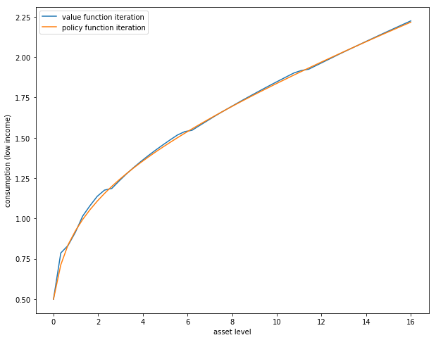
The figure shows consumption policies computed by iteration of \(K\) and \(T\) respectively
In the case of iteration with \(T\), the final value function is used to compute the observed policy.
Consumption is shown as a function of assets with income \(z\) held fixed at its smallest value.
The following details are needed to replicate the figure
The parameters are the default parameters in the definition of
consumer_problem.The initial conditions are the default ones from
initialize(cp).Both operators are iterated 80 times.
When you run your code you will observe that iteration with \(K\) is faster than iteration with \(T\).
In the Julia console, a comparison of the operators can be made as follows
cp = consumer_problem()
v, c = initialize(cp)
([-17.328679513998615 0.0; -4.664387247760648 7.125637140580436; … ; 69.82541010621486 70.57937835479346; 70.32526591846735 71.06452735149534], [0.5 1.0; 0.8297959183673469 1.329795918367347; … ; 16.33020408163265 16.83020408163265; 16.66 17.16])
@btime T(cp, v);
226.688 μs
(8201 allocations: 328.50 KiB)
@btime K(cp, c);
313.449 μs
(15459 allocations: 612.02 KiB)
42.4.2. Exercise 2#
Next let’s consider how the interest rate affects consumption.
Reproduce the following figure, which shows (approximately) optimal consumption policies for different interest rates
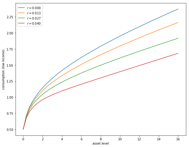
Other than r, all parameters are at their default values
r steps through range(0, 0.04, length = 4)
Consumption is plotted against assets for income shock fixed at the smallest value
The figure shows that higher interest rates boost savings and hence suppress consumption.
42.4.3. Exercise 3#
Now let’s consider the long run asset levels held by households.
We’ll take r = 0.03 and otherwise use default parameters.
The following figure is a 45 degree diagram showing the law of motion for assets when consumption is optimal
# solve for optimal consumption
m = consumer_problem(r = 0.03, grid_max = 4)
v_init, c_init = initialize(m)

sol = fixedpoint(c -> K(m, c), c_init)
c = sol.zero

a = m.asset_grid
R, z_vals = m.R, m.z_vals

# generate savings plot
plot(a, R * a .+ z_vals[1] - c[:, 1], label = "Low income")
plot!(xlabel = "Current assets", ylabel = "Next period assets")
plot!(a, R * a .+ z_vals[2] - c[:, 2], label = "High income")
plot!(xlabel = "Current assets", ylabel = "Next period assets")
plot!(a, a, linestyle = :dash, color = "black", label = "")
plot!(xlabel = "Current assets", ylabel = "Next period assets")
plot!(legend = :topleft)

The blue line and orange line represent the function
when income \(z\) takes its high and low values respectively.
The dashed line is the 45 degree line.
We can see from the figure that the dynamics will be stable — assets do not diverge.
In fact there is a unique stationary distribution of assets that we can calculate by simulation
Can be proved via theorem 2 of [HP92].
Represents the long run dispersion of assets across households when households have idiosyncratic shocks.
Ergodicity is valid here, so stationary probabilities can be calculated by averaging over a single long time series.
Hence to approximate the stationary distribution we can simulate a long time series for assets and histogram, as in the following figure
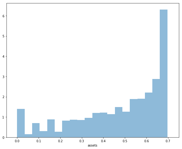
Your task is to replicate the figure
Parameters are as discussed above
The histogram in the figure used a single time series \(\{a_t\}\) of length 500,000
Given the length of this time series, the initial condition \((a_0, z_0)\) will not matter
You might find it helpful to represent the income process as a Markov chain via its transition matrix \(\Pi\) and simulate state indices directly
42.4.4. Exercise 4#
Following on from exercises 2 and 3, let’s look at how savings and aggregate asset holdings vary with the interest rate
Note: [LS18] section 18.6 can be consulted for more background on the topic treated in this exercise
For a given parameterization of the model, the mean of the stationary distribution can be interpreted as aggregate capital in an economy with a unit mass of ex-ante identical households facing idiosyncratic shocks.
Let’s look at how this measure of aggregate capital varies with the interest rate and borrowing constraint.
The next figure plots aggregate capital against the interest rate for b in (1, 3)
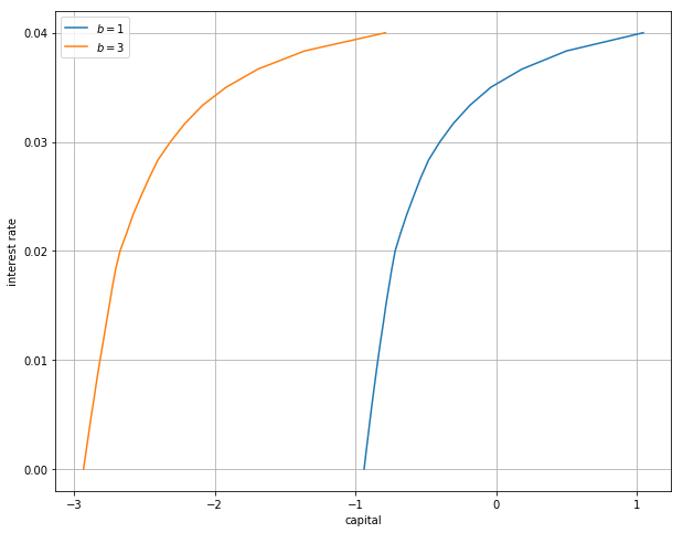
As is traditional, the price (interest rate) is on the vertical axis.
The horizontal axis is aggregate capital computed as the mean of the stationary distribution.
Exercise 4 is to replicate the figure, making use of code from previous exercises.
Try to explain why the measure of aggregate capital is equal to \(-b\) when \(r=0\) for both cases shown here.
42.5. Solutions#
42.5.1. Exercise 1#
cp = consumer_problem()
N = 80

V, c = initialize(cp)
println("Starting value function iteration")
for i in 1:N
    V = T(cp, V)
end
c1 = T(cp, V, ret_policy = true)

V2, c2 = initialize(cp)
println("Starting policy function iteration")
for i in 1:N
    c2 = K(cp, c2)
end

plot(cp.asset_grid, c1[:, 1], label = "value function iteration")
plot!(cp.asset_grid, c2[:, 1], label = "policy function iteration")
plot!(xlabel = "asset level", ylabel = "Consumption (low income)")
plot!(legend = :topleft)
Starting value function iteration
Starting policy function iteration

42.5.2. Exercise 2#
r_vals = range(0, 0.04, length = 4)
traces = []
legends = []

for r_val in r_vals
    cp = consumer_problem(r = r_val)
    v_init, c_init = initialize(cp)
    sol = fixedpoint(x -> K(cp, x), c_init)
    c = sol.zero

    traces = push!(traces, c[:, 1])
    legends = push!(legends, L"r = %$(round(r_val, digits = 3))")
end

plot(traces, label = reshape(legends, 1, length(legends)))
plot!(xlabel = "asset level", ylabel = "Consumption (low income)")
plot!(legend = :topleft)

42.5.3. Exercise 3#
function compute_asset_series(cp, T = 500_000; verbose = false)
    (; Pi, z_vals, R) = cp  # simplify names
    z_idx = 1:length(z_vals)
    v_init, c_init = initialize(cp)

    sol = fixedpoint(x -> K(cp, x), c_init)
    c = sol.zero

    cf = LinearInterpolation((cp.asset_grid, z_idx), c;
                             extrapolation_bc = Interpolations.Flat())

    a = zeros(T + 1)
    function simulate_markov_chain(P, X_0, T)
        N = size(P, 1)
        num_chains = length(X_0)
        P_dist = [Categorical(P[i, :]) for i in 1:N]
        X = zeros(Int, num_chains, T + 1)
        X[:, 1] .= X_0
        for t in 1:T
            for n in 1:num_chains
                X[n, t + 1] = rand(P_dist[X[n, t]])
            end
        end
        return X
    end

    z_seq = vec(simulate_markov_chain(Pi, [1], T))
    for t in 1:T
        i_z = z_seq[t]
        a[t + 1] = R * a[t] + z_vals[i_z] - cf(a[t], i_z)
    end
    return a
end

cp = consumer_problem(r = 0.03, grid_max = 4)
Random.seed!(42) # for reproducibility
a = compute_asset_series(cp)
histogram(a, nbins = 20, leg = false, normed = true, xlabel = "assets")

42.5.4. Exercise 4#
M = 25
r_vals = range(0, 0.04, length = M)

xs = []
ys = []
legends = []
for b in [1.0, 3.0]
    asset_mean = zeros(M)
    for (i, r_val) in enumerate(r_vals)
        cp = consumer_problem(r = r_val, b = b)
        the_mean = mean(compute_asset_series(cp, 250_000))
        asset_mean[i] = the_mean
    end
    xs = push!(xs, asset_mean)
    ys = push!(ys, r_vals)
    legends = push!(legends, L"b = %$b")
    println("Finished iteration b = $b")
end
plot(xs, ys, label = reshape(legends, 1, length(legends)))
plot!(xlabel = "capital", ylabel = "interest rate", yticks = ([0, 0.045]))
plot!(legend = :bottomright)
Finished iteration b = 1.0
Finished iteration b = 3.0
