43. Discrete State Dynamic Programming #

Contents

Discrete State Dynamic Programming

43.1. Overview #

In this lecture we discuss a family of dynamic programming problems with the following features:

a discrete state space and discrete choices (actions)
an infinite horizon
discounted rewards
Markov state transitions

We call such problems discrete dynamic programs, or discrete DPs.

Discrete DPs are the workhorses in much of modern quantitative economics, including

monetary economics
search and labor economics
household savings and consumption theory
investment theory
asset pricing
industrial organization, etc.

When a given model is not inherently discrete, it is common to replace it with a discretized version in order to use discrete DP techniques.

This lecture covers

the theory of dynamic programming in a discrete setting, plus examples and applications
a powerful set of routines for solving discrete DPs from the QuantEcon code libary

43.1.1. How to Read this Lecture#

We use dynamic programming many applied lectures, such as

The objective of this lecture is to provide a more systematic and theoretical treatment, including algorithms and implementation, while focusing on the discrete case.

43.1.2. References#

For background reading on dynamic programming and additional applications, see, for example,

[LS18]
[HLL96], section 3.5
[Put05]
[SLP89]
[Rus96]
[MF02]
EDTC, chapter 5

43.2. Discrete DPs #

Loosely speaking, a discrete DP is a maximization problem with an objective function of the form

(43.1)#\[\mathbb{E} \sum_{t = 0}^{\infty} \beta^t r(s_t, a_t)\]

where

\(s_t\) is the state variable
\(a_t\) is the action
\(\beta\) is a discount factor
\(r(s_t, a_t)\) is interpreted as a current reward when the state is \(s_t\) and the action chosen is \(a_t\)

Each pair \((s_t, a_t)\) pins down transition probabilities \(Q(s_t, a_t, s_{t+1})\) for the next period state \(s_{t+1}\).

Thus, actions influence not only current rewards but also the future time path of the state.

The essence of dynamic programming problems is to trade off current rewards vs favorable positioning of the future state (modulo randomness).

Examples:

consuming today vs saving and accumulating assets
accepting a job offer today vs seeking a better one in the future
exercising an option now vs waiting

43.2.1. Policies#

The most fruitful way to think about solutions to discrete DP problems is to compare policies.

In general, a policy is a randomized map from past actions and states to current action.

In the setting formalized below, it suffices to consider so-called stationary Markov policies, which consider only the current state.

In particular, a stationary Markov policy is a map \(\sigma\) from states to actions

\(a_t = \sigma(s_t)\) indicates that \(a_t\) is the action to be taken in state \(s_t\)

It is known that, for any arbitrary policy, there exists a stationary Markov policy that dominates it at least weakly.

See section 5.5 of [Put05] for discussion and proofs.

In what follows, stationary Markov policies are referred to simply as policies.

The aim is to find an optimal policy, in the sense of one that maximizes (43.1).

Let’s now step through these ideas more carefully.

43.2.2. Formal definition#

Formally, a discrete dynamic program consists of the following components:

A finite set of states \(S = \{0, \ldots, n-1\}\)
A finite set of feasible actions \(A(s)\) for each state \(s \in S\), and a corresponding set of feasible state-action pairs

\[ \mathit{SA} := \{(s, a) \mid s \in S, \; a \in A(s)\} \]
A reward function \(r\colon \mathit{SA} \to \mathbb{R}\)
A transition probability function \(Q\colon \mathit{SA} \to \Delta(S)\), where \(\Delta(S)\) is the set of probability distributions over \(S\)
A discount factor \(\beta \in [0, 1)\)

We also use the notation \(A := \bigcup_{s \in S} A(s) = \{0, \ldots, m-1\}\) and call this set the action space.

A policy is a function \(\sigma\colon S \to A\).

A policy is called feasible if it satisfies \(\sigma(s) \in A(s)\) for all \(s \in S\).

Denote the set of all feasible policies by \(\Sigma\).

If a decision maker uses a policy \(\sigma \in \Sigma\), then

the current reward at time \(t\) is \(r(s_t, \sigma(s_t))\)
the probability that \(s_{t+1} = s'\) is \(Q(s_t, \sigma(s_t), s')\)

For each \(\sigma \in \Sigma\), define

\(r_{\sigma}\) by \(r_{\sigma}(s) := r(s, \sigma(s))\))
\(Q_{\sigma}\) by \(Q_{\sigma}(s, s') := Q(s, \sigma(s), s')\)

Notice that \(Q_\sigma\) is a stochastic matrix on \(S\).

It gives transition probabilities of the controlled chain when we follow policy \(\sigma\).

If we think of \(r_\sigma\) as a column vector, then so is \(Q_\sigma^t r_\sigma\), and the \(s\)-th row of the latter has the interpretation

(43.2)#\[(Q_\sigma^t r_\sigma)(s) = \mathbb E [ r(s_t, \sigma(s_t)) \mid s_0 = s ] \quad \text{when } \{s_t\} \sim Q_\sigma\]

Comments

\(\{s_t\} \sim Q_\sigma\) means that the state is generated by stochastic matrix \(Q_\sigma\)
See this discussion on computing expectations of Markov chains for an explanation of the expression in (43.2)

Notice that we’re not really distinguishing between functions from \(S\) to \(\mathbb R\) and vectors in \(\mathbb R^n\).

This is natural because they are in one to one correspondence.

43.2.3. Value and Optimality#

Let \(v_{\sigma}(s)\) denote the discounted sum of expected reward flows from policy \(\sigma\) when the initial state is \(s\).

To calculate this quantity we pass the expectation through the sum in (43.1) and use (43.2) to get

\[ v_{\sigma}(s) = \sum_{t=0}^{\infty} \beta^t (Q_{\sigma}^t r_{\sigma})(s) \qquad (s \in S) \]

This function is called the policy value function for the policy \(\sigma\).

The optimal value function, or simply value function, is the function \(v^*\colon S \to \mathbb{R}\) defined by

\[ v^*(s) = \max_{\sigma \in \Sigma} v_{\sigma}(s) \qquad (s \in S) \]

(We can use max rather than sup here because the domain is a finite set)

A policy \(\sigma \in \Sigma\) is called optimal if \(v_{\sigma}(s) = v^*(s)\) for all \(s \in S\).

Given any \(w \colon S \to \mathbb R\), a policy \(\sigma \in \Sigma\) is called \(w\)-greedy if

\[ \sigma(s) \in \operatorname*{arg\,max}_{a \in A(s)} \left\{ r(s, a) + \beta \sum_{s' \in S} w(s') Q(s, a, s') \right\} \qquad (s \in S) \]

As discussed in detail below, optimal policies are precisely those that are \(v^*\)-greedy.

43.2.4. Two Operators#

It is useful to define the following operators:

The Bellman operator \(T\colon \mathbb{R}^S \to \mathbb{R}^S\) is defined by

\[ (T v)(s) = \max_{a \in A(s)} \left\{ r(s, a) + \beta \sum_{s' \in S} v(s') Q(s, a, s') \right\} \qquad (s \in S) \]

For any policy function \(\sigma \in \Sigma\), the operator \(T_{\sigma}\colon \mathbb{R}^S \to \mathbb{R}^S\) is defined by

\[ (T_{\sigma} v)(s) = r(s, \sigma(s)) + \beta \sum_{s' \in S} v(s') Q(s, \sigma(s), s') \qquad (s \in S) \]

This can be written more succinctly in operator notation as

\[ T_{\sigma} v = r_{\sigma} + \beta Q_{\sigma} v \]

The two operators are both monotone

\(v \leq w\) implies \(Tv \leq Tw\) pointwise on \(S\), and similarly for \(T_\sigma\)

They are also contraction mappings with modulus \(\beta\)

\(\lVert Tv - Tw \rVert \leq \beta \lVert v - w \rVert\) and similarly for \(T_\sigma\), where \(\lVert \cdot\rVert\) is the max norm

For any policy \(\sigma\), its value \(v_{\sigma}\) is the unique fixed point of \(T_{\sigma}\).

For proofs of these results and those in the next section, see, for example, EDTC, chapter 10.

43.2.5. The Bellman Equation and the Principle of Optimality#

The main principle of the theory of dynamic programming is that

the optimal value function \(v^*\) is a unique solution to the Bellman equation,

\[ v(s) = \max_{a \in A(s)} \left\{ r(s, a) + \beta \sum_{s' \in S} v(s') Q(s, a, s') \right\} \qquad (s \in S), \]

or in other words, \(v^*\) is the unique fixed point of \(T\), and
\(\sigma^*\) is an optimal policy function if and only if it is \(v^*\)-greedy

By the definition of greedy policies given above, this means that

\[ \sigma^*(s) \in \operatorname*{arg\,max}_{a \in A(s)} \left\{ r(s, a) + \beta \sum_{s' \in S} v^*(s') Q(s, a, s') \right\} \qquad (s \in S) \]

43.3. Solving Discrete DPs #

Now that the theory has been set out, let’s turn to solution methods.

Code for solving discrete DPs is available in ddp.jl from the QuantEcon.jl code library.

It implements the three most important solution methods for discrete dynamic programs, namely

value function iteration
policy function iteration
modified policy function iteration

Let’s briefly review these algorithms and their implementation.

43.3.1. Value Function Iteration#

Perhaps the most familiar method for solving all manner of dynamic programs is value function iteration.

This algorithm uses the fact that the Bellman operator \(T\) is a contraction mapping with fixed point \(v^*\).

Hence, iterative application of \(T\) to any initial function \(v^0 \colon S \to \mathbb R\) converges to \(v^*\).

The details of the algorithm can be found in the appendix.

43.3.2. Policy Function Iteration#

This routine, also known as Howard’s policy improvement algorithm, exploits more closely the particular structure of a discrete DP problem.

Each iteration consists of

A policy evaluation step that computes the value \(v_{\sigma}\) of a policy \(\sigma\) by solving the linear equation \(v = T_{\sigma} v\).
A policy improvement step that computes a \(v_{\sigma}\)-greedy policy.

In the current setting policy iteration computes an exact optimal policy in finitely many iterations.

See theorem 10.2.6 of EDTC for a proof

The details of the algorithm can be found in the appendix.

43.3.3. Modified Policy Function Iteration#

Modified policy iteration replaces the policy evaluation step in policy iteration with “partial policy evaluation”.

The latter computes an approximation to the value of a policy \(\sigma\) by iterating \(T_{\sigma}\) for a specified number of times.

This approach can be useful when the state space is very large and the linear system in the policy evaluation step of policy iteration is correspondingly difficult to solve.

The details of the algorithm can be found in the appendix.

43.4. Example: A Growth Model #

Let’s consider a simple consumption-saving model.

A single household either consumes or stores its own output of a single consumption good.

The household starts each period with current stock \(s\).

Next, the household chooses a quantity \(a\) to store and consumes \(c = s - a\)

Storage is limited by a global upper bound \(M\)
Flow utility is \(u(c) = c^{\alpha}\)

Output is drawn from a discrete uniform distribution on \(\{0, \ldots, B\}\).

The next period stock is therefore

\[ s' = a + U \quad \text{where} \quad U \sim U[0, \ldots, B] \]

The discount factor is \(\beta \in [0, 1)\).

43.4.1. Discrete DP Representation#

We want to represent this model in the format of a discrete dynamic program.

To this end, we take

the state variable to be the stock \(s\)
the state space to be \(S = \{0, \ldots, M + B\}\)
- hence \(n = M + B + 1\)
the action to be the storage quantity \(a\)
the set of feasible actions at \(s\) to be \(A(s) = \{0, \ldots, \min\{s, M\}\}\)
- hence \(A = \{0, \ldots, M\}\) and \(m = M + 1\)
the reward function to be \(r(s, a) = u(s - a)\)
the transition probabilities to be

(43.3)#\[\begin{split}Q(s, a, s') := \begin{cases} \frac{1}{B + 1} & \text{if } a \leq s' \leq a + B \\ 0 & \text{ otherwise} \end{cases}\end{split}\]

43.4.2. Defining a DiscreteDP Instance#

This information will be used to create an instance of DiscreteDP by passing the following information

An \(n \times m\) reward array \(R\)
An \(n \times m \times n\) transition probability array \(Q\)
A discount factor \(\beta\)

For \(R\) we set \(R[s, a] = u(s - a)\) if \(a \leq s\) and \(-\infty\) otherwise.

For \(Q\) we follow the rule in (43.3).

Note:

The feasibility constraint is embedded into \(R\) by setting \(R[s, a] = -\infty\) for \(a \notin A(s)\).
Probability distributions for \((s, a)\) with \(a \notin A(s)\) can be arbitrary.

The following code sets up these objects for us.

using BenchmarkTools, LaTeXStrings, LinearAlgebra, Plots, QuantEcon, Statistics
using SparseArrays

using BenchmarkTools, Plots, QuantEcon

SimpleOG(; B = 10, M = 5, alpha = 0.5, beta = 0.9) = (; B, M, alpha, beta)

function transition_matrices(g)
    (; B, M, alpha, beta) = g
    u(c) = c^alpha
    n = B + M + 1
    m = M + 1

    R = zeros(n, m)
    Q = zeros(n, m, n)

    for a in 0:M
        Q[:, a + 1, (a:(a + B)) .+ 1] .= 1 / (B + 1)
        for s in 0:(B + M)
            R[s + 1, a + 1] = (a <= s ? u(s - a) : -Inf)
        end
    end

    return (; Q, R)
end

transition_matrices (generic function with 1 method)

Let’s run this code and create an instance of SimpleOG

g = SimpleOG();
Q, R = transition_matrices(g);

In case the preceding code was too concise, we can see a more verbose form

function verbose_matrices(g)
    (;B, M, alpha, beta) = g
    u(c) = c^alpha

    #Matrix dimensions. The +1 is due to the 0 state.
    n = B + M + 1
    m = M + 1

    R = fill(-Inf, n, m) #Start assuming nothing is feasible
    Q = zeros(n,m,n) #Assume 0 by default

    #Create the R matrix
    #Note: indexing into matrix complicated since Julia starts indexing at 1 instead of 0
    #but the state s and choice a can be 0
    for a in 0:M
         for s in 0:(B + M)
            if a <= s #i.e. if feasible
                R[s + 1, a + 1] = u(s - a)
            end
        end
    end

    #Create the Q multi-array
    for s in 0:(B+M) #For each state
        for a in 0:M #For each action
            for sp in 0:(B+M) #For each state next period
                if( sp >= a && sp <= a + B) # The support of all realizations
                    Q[s + 1, a + 1, sp + 1] = 1 / (B + 1) # Same prob of all
                end
            end
            @assert sum(Q[s + 1, a + 1, :]) ≈ 1 #Optional check that matrix is stochastic
         end
    end
return (;Q,R)
end

verbose_matrices (generic function with 1 method)

Instances of DiscreteDP are created using the signature DiscreteDP(R, Q, beta).

Let’s create an instance using the objects stored in g

ddp = DiscreteDP(R, Q, g.beta);

Now that we have an instance ddp of DiscreteDP we can solve it as follows

results = solve(ddp, PFI)

QuantEcon.DPSolveResult{PFI, Float64}([19.017402216959916, 20.017402216959912, 20.431615779333015, 20.749453024528794, 21.040780991093484, 21.30873018352461, 21.544798161024396, 21.769281810799857, 21.982703576083246, 22.188243228238495, 22.38450479651991, 22.578077363861723, 22.76109126977111, 22.94376708345271, 23.115339958706524, 23.277617618874903], [19.017402216959916, 20.017402216959916, 20.43161577933301, 20.749453024528794, 21.040780991093488, 21.30873018352461, 21.5447981610244, 21.769281810799864, 21.982703576083253, 22.1882432282385, 22.38450479651991, 22.578077363861723, 22.76109126977111, 22.943767083452713, 23.11533995870652, 23.2776176188749], 3, [1, 1, 1, 1, 2, 2, 2, 3, 3, 4, 4, 5, 6, 6, 6, 6], Discrete Markov Chain
stochastic matrix of type Adjoint{Float64, Matrix{Float64}}:
[0.09090909090909091 0.09090909090909091 … 0.0 0.0; 0.09090909090909091 0.09090909090909091 … 0.0 0.0; … ; 0.0 0.0 … 0.09090909090909091 0.09090909090909091; 0.0 0.0 … 0.09090909090909091 0.09090909090909091])

Let’s see what we’ve got here

fieldnames(typeof(results))

(:v, :Tv, :num_iter, :sigma, :mc)

The most important attributes are v, the value function, and sigma, the optimal policy

results.v

16-element Vector{Float64}:
017402216959916
017402216959912
431615779333015
749453024528794
040780991093484
30873018352461
544798161024396
769281810799857
982703576083246
188243228238495
38450479651991
578077363861723
76109126977111
94376708345271
115339958706524
277617618874903

results.sigma .- 1

16-element Vector{Int64}:
 0
 0
 0
 0
 1
 1
 1
 2
 2
 3
 3
 4
 5
 5
 5
 5

Here 1 is subtracted from results.sigma because we added 1 to each state and action to create valid indices.

Since we’ve used policy iteration, these results will be exact unless we hit the iteration bound max_iter.

Let’s make sure this didn’t happen

results.num_iter

In this case we converged in only 3 iterations.

Another interesting object is results.mc, which is the controlled chain defined by \(Q_{\sigma^*}\), where \(\sigma^*\) is the optimal policy.

In other words, it gives the dynamics of the state when the agent follows the optimal policy.

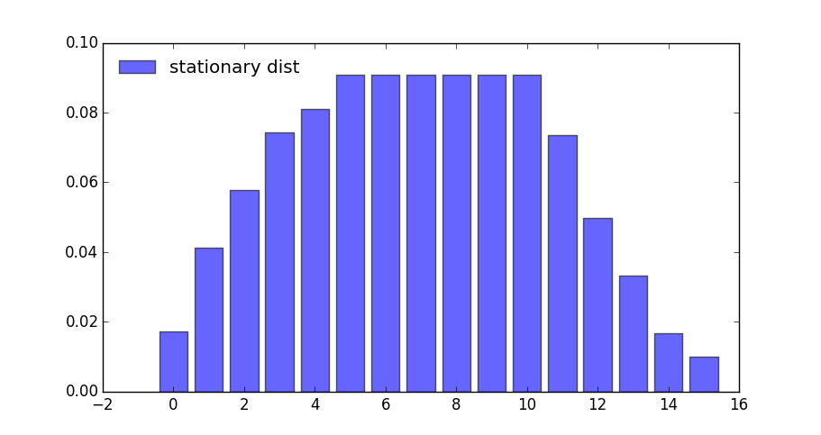
Since this object is an instance of MarkovChain from QuantEcon.jl (see this lecture for more discussion), we can easily simulate it, compute its stationary distribution and so on

stationary_distributions(results.mc)[1]

16-element Vector{Float64}:
01732186732186732
041210632119723034
05773955773955773
07426848335939244
08095823095823096
09090909090909091
0909090909090909
0909090909090909
09090909090909093
09090909090909091
09090909090909091
0735872235872236
049698458789367884
033169533169533166
016640607549698462
009950859950859951

Here’s the same information in a bar graph

What happens if the agent is more patient?

g_2 = SimpleOG(beta = 0.99);
Q_2, R_2 = transition_matrices(g_2);

ddp_2 = DiscreteDP(R_2, Q_2, g_2.beta)

results_2 = solve(ddp_2, PFI)

std_2 = stationary_distributions(results_2.mc)[1]

16-element Vector{Float64}:
005469129800680602
023213417598444343
03147788040836169
04800680602819641
056271268838113765
09090909090909091
09090909090909093
09090909090909093
09090909090909094
09090909090909093
09090909090909094
0854399611084103
06769567331064659
059431210500729234
042902284880894495
03463782207097716

bar(std_2, label = "stationary dist")

We can see the rightward shift in probability mass.

43.4.3. State-Action Pair Formulation#

The DiscreteDP type in fact provides a second interface to setting up an instance.

One of the advantages of this alternative set up is that it permits use of a sparse matrix for Q.

(An example of using sparse matrices is given in the exercises below)

The call signature of the second formulation is DiscreteDP(R, Q, beta, s_indices, a_indices) where

s_indices and a_indices are arrays of equal length L enumerating all feasible state-action pairs
R is an array of length L giving corresponding rewards
Q is an L x n transition probability array

Here’s how we could set up these objects for the preceding example

B = 10
M = 5
alpha = 0.5
beta = 0.9
u(c) = c^alpha
n = B + M + 1
m = M + 1

s_indices = Int64[]
a_indices = Int64[]
Q = zeros(0, n)
R = zeros(0)

b = 1 / (B + 1)

for s in 0:(M + B)
    for a in 0:min(M, s)
        s_indices = [s_indices; s + 1]
        a_indices = [a_indices; a + 1]
        q = zeros(1, n)
        q[(a + 1):((a + B) + 1)] .= b
        Q = [Q; q]
        R = [R; u(s - a)]
    end
end

ddp = DiscreteDP(R, Q, beta, s_indices, a_indices);
results = solve(ddp, PFI)

QuantEcon.DPSolveResult{PFI, Float64}([19.017402216959916, 20.017402216959912, 20.431615779333015, 20.749453024528794, 21.040780991093484, 21.30873018352461, 21.544798161024396, 21.769281810799857, 21.982703576083246, 22.188243228238495, 22.38450479651991, 22.578077363861723, 22.76109126977111, 22.94376708345271, 23.115339958706524, 23.277617618874903], [19.017402216959916, 20.017402216959916, 20.43161577933301, 20.749453024528794, 21.040780991093488, 21.30873018352461, 21.5447981610244, 21.769281810799864, 21.982703576083253, 22.1882432282385, 22.38450479651991, 22.578077363861723, 22.76109126977111, 22.943767083452713, 23.11533995870652, 23.2776176188749], 3, [1, 1, 1, 1, 2, 2, 2, 3, 3, 4, 4, 5, 6, 6, 6, 6], Discrete Markov Chain
stochastic matrix of type Matrix{Float64}:
[0.09090909090909091 0.09090909090909091 … 0.0 0.0; 0.09090909090909091 0.09090909090909091 … 0.0 0.0; … ; 0.0 0.0 … 0.09090909090909091 0.09090909090909091; 0.0 0.0 … 0.09090909090909091 0.09090909090909091])

43.5. Exercises #

In the stochastic optimal growth lecture dynamic programming lecture, we solve a benchmark model that has an analytical solution to check we could replicate it numerically.

The exercise is to replicate this solution using DiscreteDP.

43.6. Solutions #

These were written jointly by Max Huber and Daisuke Oyama.

43.6.1. Setup#

Details of the model can be found in the lecture. As in the lecture, we let \(f(k) = k^{\alpha}\) with \(\alpha = 0.65\), \(u(c) = \log c\), and \(\beta = 0.95\).

alpha = 0.65
f(k) = k .^ alpha
u_log(x) = log(x)
beta = 0.95

0.95

Here we want to solve a finite state version of the continuous state model above. We discretize the state space into a grid of size grid_size = 500, from \(10^{-6}\) to grid_max=2.

grid_max = 2
grid_size = 500
grid = range(1e-6, grid_max, length = grid_size)

1.0e-6:0.004008014028056112:2.0

We choose the action to be the amount of capital to save for the next period (the state is the capital stock at the beginning of the period). Thus the state indices and the action indices are both 1, …, grid_size. Action (indexed by) a is feasible at state (indexed by) s if and only if grid[a] < f([grid[s]) (zero consumption is not allowed because of the log utility).

Thus the Bellman equation is:

\[ v(k) = \max_{0 < k' < f(k)} u(f(k) - k') + \beta v(k'), \]

where \(k^{\prime}\) is the capital stock in the next period.

The transition probability array Q will be highly sparse (in fact it is degenerate as the model is deterministic), so we formulate the problem with state-action pairs, to represent Q in sparse matrix format.

We first construct indices for state-action pairs:

C = f.(grid) .- grid'
coord = repeat(collect(1:grid_size), 1, grid_size) #coordinate matrix
s_indices = coord[C .> 0]
a_indices = transpose(coord)[C .> 0]
L = length(a_indices)

Now let’s set up \(R\) and \(Q\)

R = u_log.(C[C .> 0]);

using SparseArrays

Q = spzeros(L, grid_size) # Formerly spzeros

for i in 1:L
    Q[i, a_indices[i]] = 1
end

We’re now in a position to create an instance of DiscreteDP corresponding to the growth model.

ddp = DiscreteDP(R, Q, beta, s_indices, a_indices);

43.6.2. Solving the Model#

results = solve(ddp, PFI)
v, sigma, num_iter = results.v, results.sigma, results.num_iter
num_iter

Let us compare the solution of the discrete model with the exact solution of the original continuous model. Here’s the exact solution:

c = f(grid) - grid[sigma]

ab = alpha * beta
c1 = (log(1 - alpha * beta) + log(alpha * beta) * alpha * beta / (1 - alpha * beta)) /
     (1 - beta)
c2 = alpha / (1 - alpha * beta)

v_star(k) = c1 + c2 * log(k)
c_star(k) = (1 - alpha * beta) * k .^ alpha

c_star (generic function with 1 method)

Let’s plot the value functions.

plot(grid, [v v_star.(grid)], ylim = (-40, -32), lw = 2,
     label = ["discrete" "continuous"])

They are barely distinguishable (although you can see the difference if you zoom).

Now let’s look at the discrete and exact policy functions for consumption.

plot(grid, [c c_star.(grid)], lw = 2, label = ["discrete" "continuous"],
     legend = :topleft)

These functions are again close, although some difference is visible and becomes more obvious as you zoom. Here are some statistics:

maximum(abs(x - v_star(y)) for (x, y) in zip(v, grid))

121.49819147053378

This is a big error, but most of the error occurs at the lowest gridpoint. Otherwise the fit is reasonable:

maximum(abs(v[idx] - v_star(grid[idx])) for idx in 2:lastindex(v))

0.012681735127500815

The value function is monotone, as expected:

all(x -> x >= 0, diff(v))

true

43.6.3. Comparison of the solution methods#

Let’s try different solution methods. The results below show that policy function iteration and modified policy function iteration are much faster than value function iteration.

@benchmark results = solve(ddp, PFI)
results = solve(ddp, PFI);

@benchmark res1 = solve(ddp, VFI, max_iter = 500, epsilon = 1e-4)
res1 = solve(ddp, VFI, max_iter = 500, epsilon = 1e-4);

res1.num_iter

sigma == res1.sigma

true

@benchmark res2 = solve(ddp, MPFI, max_iter = 500, epsilon = 1e-4)
res2 = solve(ddp, MPFI, max_iter = 500, epsilon = 1e-4);

res2.num_iter

sigma == res2.sigma

true

43.6.4. Replication of the figures#

Let’s visualize convergence of value function iteration, as in the lecture.

w_init = 5log.(grid) .- 25  # Initial condition
n = 50

ws = []
colors = []
w = w_init
for i in 0:(n - 1)
    w = bellman_operator(ddp, w)
    push!(ws, w)
    push!(colors, RGBA(0, 0, 0, i / n))
end

plot(grid,
     w_init,
     ylims = (-40, -20),
     lw = 2,
     xlims = extrema(grid),
     label = "initial condition")

plot!(grid, ws, label = "", color = reshape(colors, 1, length(colors)), lw = 2)
plot!(grid, v_star.(grid), label = "true value function", color = :red, lw = 2)

We next plot the consumption policies along the value iteration. First we write a function to generate and record the policies at given stages of iteration.

function compute_policies(n_vals...)
    c_policies = []
    w = w_init
    for n in 1:maximum(n_vals)
        w = bellman_operator(ddp, w)
        if n in n_vals
            sigma = compute_greedy(ddp, w)
            c_policy = f(grid) - grid[sigma]
            push!(c_policies, c_policy)
        end
    end
    return c_policies
end

compute_policies (generic function with 1 method)

Now let’s generate the plots.

true_c = c_star.(grid)
c_policies = compute_policies(2, 4, 6)
plot_vecs = [c_policies[1] c_policies[2] c_policies[3] true_c true_c true_c]
l1 = "approximate optimal policy"
l2 = "optimal consumption policy"
labels = [l1 l1 l1 l2 l2 l2]
plot(grid,
     plot_vecs,
     xlim = (0, 2),
     ylim = (0, 1),
     layout = (3, 1),
     lw = 2,
     label = labels,
     size = (600, 800),
     title = ["2 iterations" "4 iterations" "6 iterations"])

43.6.5. Dynamics of the capital stock#

Finally, let us work on Exercise 2, where we plot the trajectories of the capital stock for three different discount factors, \(0.9\), \(0.94\), and \(0.98\), with initial condition \(k_0 = 0.1\).

discount_factors = (0.9, 0.94, 0.98)
k_init = 0.1

k_init_ind = findfirst(collect(grid) .>= k_init)

sample_size = 25

ddp0 = DiscreteDP(R, Q, beta, s_indices, a_indices)
k_paths = []
labels = []

for beta in discount_factors
    ddp0.beta = beta
    res0 = solve(ddp0, PFI)
    k_path_ind = simulate(res0.mc, sample_size, init = k_init_ind)
    k_path = grid[k_path_ind .+ 1]
    push!(k_paths, k_path)
    push!(labels, L"\beta = %$beta")
end

plot(k_paths,
     xlabel = "time",
     ylabel = "capital",
     ylim = (0.1, 0.3),
     lw = 2,
     markershape = :circle,
     label = reshape(labels, 1, length(labels)))

43.7. Appendix: Algorithms #

This appendix covers the details of the solution algorithms implemented for DiscreteDP.

We will make use of the following notions of approximate optimality:

For \(\varepsilon > 0\), \(v\) is called an \(\varepsilon\)-approximation of \(v^*\) if \(\lVert v - v^*\rVert < \varepsilon\)
A policy \(\sigma \in \Sigma\) is called \(\varepsilon\)-optimal if \(v_{\sigma}\) is an \(\varepsilon\)-approximation of \(v^*\)

43.7.1. Value Iteration#

The DiscreteDP value iteration method implements value function iteration as follows

Choose any \(v^0 \in \mathbb{R}^n\), and specify \(\varepsilon > 0\); set \(i = 0\).
Compute \(v^{i+1} = T v^i\).
If \(\lVert v^{i+1} - v^i\rVert < [(1 - \beta) / (2\beta)] \varepsilon\), then go to step 4; otherwise, set \(i = i + 1\) and go to step 2.
Compute a \(v^{i+1}\)-greedy policy \(\sigma\), and return \(v^{i+1}\) and \(\sigma\).

Given \(\varepsilon > 0\), the value iteration algorithm

terminates in a finite number of iterations
returns an \(\varepsilon/2\)-approximation of the optimal value function and an \(\varepsilon\)-optimal policy function (unless iter_max is reached)

(While not explicit, in the actual implementation each algorithm is terminated if the number of iterations reaches iter_max)

43.7.2. Policy Iteration#

The DiscreteDP policy iteration method runs as follows

Choose any \(v^0 \in \mathbb{R}^n\) and compute a \(v^0\)-greedy policy \(\sigma^0\); set \(i = 0\).
Compute the value \(v_{\sigma^i}\) by solving the equation \(v = T_{\sigma^i} v\).
Compute a \(v_{\sigma^i}\)-greedy policy \(\sigma^{i+1}\); let \(\sigma^{i+1} = \sigma^i\) if possible.
If \(\sigma^{i+1} = \sigma^i\), then return \(v_{\sigma^i}\) and \(\sigma^{i+1}\); otherwise, set \(i = i + 1\) and go to step 2.

The policy iteration algorithm terminates in a finite number of iterations.

It returns an optimal value function and an optimal policy function (unless iter_max is reached).

43.7.3. Modified Policy Iteration#

The DiscreteDP modified policy iteration method runs as follows:

Choose any \(v^0 \in \mathbb{R}^n\), and specify \(\varepsilon > 0\) and \(k \geq 0\); set \(i = 0\).
Compute a \(v^i\)-greedy policy \(\sigma^{i+1}\); let \(\sigma^{i+1} = \sigma^i\) if possible (for \(i \geq 1\)).
Compute \(u = T v^i\) (\(= T_{\sigma^{i+1}} v^i\)). If \(\mathrm{span}(u - v^i) < [(1 - \beta) / \beta] \varepsilon\), then go to step 5; otherwise go to step 4.
- Span is defined by \(\mathrm{span}(z) = \max(z) - \min(z)\)
Compute \(v^{i+1} = (T_{\sigma^{i+1}})^k u\) (\(= (T_{\sigma^{i+1}})^{k+1} v^i\)); set \(i = i + 1\) and go to step 2.
Return \(v = u + [\beta / (1 - \beta)] [(\min(u - v^i) + \max(u - v^i)) / 2] \mathbf{1}\) and \(\sigma_{i+1}\).

Given \(\varepsilon > 0\), provided that \(v^0\) is such that \(T v^0 \geq v^0\), the modified policy iteration algorithm terminates in a finite number of iterations.

It returns an \(\varepsilon/2\)-approximation of the optimal value function and an \(\varepsilon\)-optimal policy function (unless iter_max is reached).

See also the documentation for DiscreteDP.