24. Finite Markov Chains#
Contents
24.1. Overview#
Markov chains are one of the most useful classes of stochastic processes, being
simple, flexible and supported by many elegant theoretical results
valuable for building intuition about random dynamic models
central to quantitative modeling in their own right
You will find them in many of the workhorse models of economics and finance.
In this lecture we review some of the theory of Markov chains. QuantEcon.jl provides routines for working with Markov chains, but we’ll stick to lightweight versions built from scratch here.
Prerequisite knowledge is basic probability and linear algebra.
using Pkg; pkgs = ["Distributions", "Graphs", "Plots"]; all(haskey.(Ref(Pkg.project().dependencies), pkgs)) || Pkg.add(pkgs)
using LinearAlgebra, Statistics
using Distributions, Random, Graphs, Plots
24.2. Definitions#
The following concepts are fundamental.
24.2.1. Stochastic Matrices#
A stochastic matrix (or Markov matrix) is an \(n \times n\) square matrix \(P\) such that
each element of \(P\) is nonnegative, and
each row of \(P\) sums to one
Each row of \(P\) can be regarded as a probability mass function over \(n\) possible outcomes.
It is not difficult to check that if \(P\) is a stochastic matrix, then so is the \(k\)-th power \(P^k\) for all \(k \in \mathbb N\).
24.2.2. Markov Chains#
There is a close connection between stochastic matrices and Markov chains.
To begin, let \(S\) be a finite set with \(n\) elements \(\{x_1, \ldots, x_n\}\).
The set \(S\) is called the state space and \(x_1, \ldots, x_n\) are the state values.
A Markov chain \(\{X_t\}\) on \(S\) is a sequence of random variables on \(S\) that have the Markov property.
This means that, for any date \(t\) and any state \(y \in S\),
In other words, knowing the current state is enough to know probabilities for future states.
In particular, the dynamics of a Markov chain are fully determined by the set of values
By construction,
\(P(x, y)\) is the probability of going from \(x\) to \(y\) in one unit of time (one step)
\(P(x, \cdot)\) is the conditional distribution of \(X_{t+1}\) given \(X_t = x\)
We can view \(P\) as a stochastic matrix where
Going the other way, if we take a stochastic matrix \(P\), we can generate a Markov chain \(\{X_t\}\) as follows:
draw \(X_0\) from some specified distribution
for each \(t = 0, 1, \ldots\), draw \(X_{t+1}\) from \(P(X_t,\cdot)\)
By construction, the resulting process satisfies (24.2).
24.2.3. Example 1#
Consider a worker who, at any given time \(t\), is either unemployed (state 1) or employed (state 2).
Suppose that, over a one month period,
An unemployed worker finds a job with probability \(\alpha \in (0, 1)\).
An employed worker loses her job and becomes unemployed with probability \(\beta \in (0, 1)\).
In terms of a Markov model, we have
\(S = \{ 1, 2\}\)
\(P(1, 2) = \alpha\) and \(P(2, 1) = \beta\)
We can write out the transition probabilities in matrix form as
Once we have the values \(\alpha\) and \(\beta\), we can address a range of questions, such as
What is the average duration of unemployment?
Over the long-run, what fraction of time does a worker find herself unemployed?
Conditional on employment, what is the probability of becoming unemployed at least once over the next 12 months?
We’ll cover such applications below.
24.2.4. Example 2#
Using US unemployment data, Hamilton [Ham05] estimated the stochastic matrix
where
the frequency is monthly
the first state represents “normal growth”
the second state represents “mild recession”
the third state represents “severe recession”
For example, the matrix tells us that when the state is normal growth, the state will again be normal growth next month with probability 0.97.
In general, large values on the main diagonal indicate persistence in the process \(\{ X_t \}\).
This Markov process can also be represented as a directed graph, with edges labeled by transition probabilities
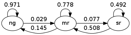
Here “ng” is normal growth, “mr” is mild recession, etc.
24.3. Simulation#
One natural way to answer questions about Markov chains is to simulate them.
(To approximate the probability of event \(E\), we can simulate many times and count the fraction of times that \(E\) occurs)
In these exercises we’ll take the state space to be \(S = 1,\ldots, n\).
24.3.1. Rolling our own#
To simulate a Markov chain, we need its stochastic matrix \(P\) and either an initial state or a probability distribution \(\psi\) for initial state to be drawn from.
The Markov chain is then constructed as discussed above. To repeat:
At time \(t=0\), the \(X_0\) is set to some fixed state or chosen from \(\psi\).
At each subsequent time \(t\), the new state \(X_{t+1}\) is drawn from \(P(X_t, \cdot)\).
In order to implement this simulation procedure, we need a method for generating draws from a discrete distributions.
For this task we’ll use a Categorical random variable (i.e. a discrete random variable with assigned probabilities)
d = Categorical([0.5, 0.3, 0.2]) # 3 discrete states
@show rand(d, 5)
@show supertype(typeof(d))
@show pdf(d, 1) # the probability to be in state 1
@show support(d)
@show pdf.(d, support(d)); # broadcast the pdf over the whole support
rand(d, 5) = [1, 3, 1, 1, 1]
supertype(typeof(d)) = Distribution{Univariate, Discrete}
pdf(d, 1) = 0.5
support(d) = Base.OneTo(3)
pdf.(d, support(d)) = [0.5, 0.3, 0.2]
We’ll write our code as a function that takes the following three arguments
A stochastic matrix
PAn initial state
initA positive integer
sample_sizerepresenting the length of the time series the function should return
function mc_sample_path(P; init = 1, sample_size = 1000)
    @assert size(P)[1] == size(P)[2] # square required
    N = size(P)[1] # should be square

    # create vector of discrete RVs for each row
    dists = [Categorical(P[i, :]) for i in 1:N]

    # setup the simulation
    X = fill(0, sample_size) # allocate memory, or zeros(Int64, sample_size)
    X[1] = init # set the initial state

    for t in 2:sample_size
        dist = dists[X[t - 1]] # get discrete RV from last state's transition distribution
        X[t] = rand(dist) # draw new value
    end
    return X
end
mc_sample_path (generic function with 1 method)
Let’s see how it works using the small matrix
As we’ll see later, for a long series drawn from P, the fraction of the sample that takes value 1 will be about 0.25.
If you run the following code you should get roughly that answer
P = [0.4 0.6; 0.2 0.8]
X = mc_sample_path(P, sample_size = 100_000); # note 100_000 = 100000
mu_1 = count(X .== 1) / length(X) # .== broadcasts test for equality. Could use mean(X .== 1)
0.24863
24.4. Marginal Distributions#
Suppose that
\(\{X_t\}\) is a Markov chain with stochastic matrix \(P\)
the distribution of \(X_t\) is known to be \(\psi_t\)
What then is the distribution of \(X_{t+1}\), or, more generally, of \(X_{t+m}\)?
24.4.1. Solution#
Let \(\psi_t\) be the distribution of \(X_t\) for \(t = 0, 1, 2, \ldots\).
Our first aim is to find \(\psi_{t + 1}\) given \(\psi_t\) and \(P\).
To begin, pick any \(y \in S\).
Using the law of total probability, we can decompose the probability that \(X_{t+1} = y\) as follows:
In words, to get the probability of being at \(y\) tomorrow, we account for all ways this can happen and sum their probabilities.
Rewriting this statement in terms of marginal and conditional probabilities gives.
There are \(n\) such equations, one for each \(y \in S\).
If we think of \(\psi_{t+1}\) and \(\psi_t\) as row vectors (as is traditional in this literature), these \(n\) equations are summarized by the matrix expression.
In other words, to move the distribution forward one unit of time, we postmultiply by \(P\).
By repeating this \(m\) times we move forward \(m\) steps into the future.
Hence, iterating on (24.5), the expression \(\psi_{t+m} = \psi_t P^m\) is also valid — here \(P^m\) is the \(m\)-th power of \(P\).
As a special case, we see that if \(\psi_0\) is the initial distribution from which \(X_0\) is drawn, then \(\psi_0 P^m\) is the distribution of \(X_m\).
This is very important, so let’s repeat it
and, more generally,
24.4.2. Multiple Step Transition Probabilities#
We know that the probability of transitioning from \(x\) to \(y\) in one step is \(P(x,y)\).
It turns out that the probability of transitioning from \(x\) to \(y\) in \(m\) steps is \(P^m(x,y)\), the \((x,y)\)-th element of the \(m\)-th power of \(P\).
To see why, consider again (24.7), but now with \(\psi_t\) putting all probability on state \(x\).
1 in the \(x\)-th position and zero elsewhere.
Inserting this into (24.7), we see that, conditional on \(X_t = x\), the distribution of \(X_{t+m}\) is the \(x\)-th row of \(P^m\).
In particular
24.4.3. Example: Probability of Recession#
Recall the stochastic matrix \(P\) for recession and growth considered above.
Suppose that the current state is unknown — perhaps statistics are available only at the end of the current month.
We estimate the probability that the economy is in state \(x\) to be \(\psi(x)\).
The probability of being in recession (either mild or severe) in 6 months time is given by the inner product
24.4.4. Example 2: Cross-Sectional Distributions#
The marginal distributions we have been studying can be viewed either as probabilities or as cross-sectional frequencies in large samples.
To illustrate, recall our model of employment / unemployment dynamics for a given worker discussed above.
Consider a large (i.e., tending to infinite) population of workers, each of whose lifetime experiences are described by the specified dynamics, independently of one another.
Let \(\psi\) be the current cross-sectional distribution over \(\{ 1, 2 \}\).
For example, \(\psi(1)\) is the unemployment rate.
The cross-sectional distribution records the fractions of workers employed and unemployed at a given moment.
The same distribution also describes the fractions of a particular worker’s career spent being employed and unemployed, respectively.
24.5. Irreducibility and Aperiodicity#
Irreducibility and aperiodicity are central concepts of modern Markov chain theory.
Let’s see what they’re about.
24.5.1. Helper functions#
Before turning to irreducibility and aperiodicity, let’s collect a few helper functions that operate directly on the transition matrix.
We rely on Graphs.jl to expose connectivity, periodicity, and stationary distributions. See here for QuantEcon.jl’s implementation.
function transition_graph(P)
    n, m = size(P)
    @assert n == m "Transition matrix must be square"
    g = DiGraph(n)
    for i in 1:n, j in 1:n
        if P[i, j] > 0
            add_edge!(g, i, j)
        end
    end
    return g
end

function communication_classes(P)
    classes = [sort!(collect(c)) for c in strongly_connected_components(transition_graph(P))]
    sort!(classes, by = first)
    return classes
end

is_irreducible(P) = length(communication_classes(P)) == 1

function state_period(P, state; max_iter = 200)
    n, m = size(P)
    @assert n == m "Transition matrix must be square"
    T = Matrix{Float64}(P)
    current = Matrix{Float64}(I, n, n)
    g = 0
    for k in 1:max_iter
        current = current * T
        if current[state, state] > 0
            g = gcd(g, k)
        end
    end
    return g
end

function period(P; max_iter = 200)
    n, m = size(P)
    @assert n == m "Transition matrix must be square"
    p = 0
    for s in 1:n
        p = gcd(p, state_period(P, s; max_iter = max_iter))
    end
    return p
end

is_aperiodic(P) = period(P) == 1

function stationary_distributions(P)
    n, m = size(P)
    @assert n == m "Transition matrix must be square"
    ev = eigen(Matrix{Float64}(P'))
    idxs = findall(λ -> isapprox(λ, 1), ev.values)
    @assert !isempty(idxs) "No unit eigenvalue found for the transition matrix"
    dists = Vector{Vector{Float64}}()
    for idx in idxs
        v = real.(ev.vectors[:, idx])
        push!(dists, vec(v ./ sum(v)))
    end
    return dists
end
stationary_distributions (generic function with 1 method)
transition_graph converts a transition matrix into a DiGraph so that we can use graph connectivity tools; Graphs.jl does not ship a dedicated helper for stochastic matrices, but the conversion is just adding directed edges wherever \(P_{ij} > 0\).
The state_period routine returns the greatest common divisor of all return times to a given state (computed up to max_iter), mirroring the definition in, e.g., the periodicity entry on Wikipedia.
By default the period calculation searches up to max_iter = 200 steps; increase it if your chain mixes slowly.
24.5.2. Irreducibility#
Let \(P\) be a fixed stochastic matrix.
Two states \(x\) and \(y\) are said to communicate with each other if there exist positive integers \(j\) and \(k\) such that
In view of our discussion above, this means precisely that
state \(x\) can be reached eventually from state \(y\), and
state \(y\) can be reached eventually from state \(x\)
The stochastic matrix \(P\) is called irreducible if all states communicate; that is, if \(x\) and \(y\) communicate for all \((x, y)\) in \(S \times S\).
For example, consider the following transition probabilities for wealth of a fictitious set of households
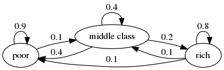
We can translate this into a stochastic matrix, putting zeros where there’s no edge between nodes
It’s clear from the graph that this stochastic matrix is irreducible: we can reach any state from any other state eventually.
We can also test this using our helper from Helper functions
P = [0.9 0.1 0.0;
     0.4 0.4 0.2;
     0.1 0.1 0.8];
is_irreducible(P)
true
Here’s a more pessimistic scenario, where the poor are poor forever
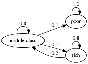
This stochastic matrix is not irreducible, since, for example, rich is not accessible from poor.
Let’s confirm this
P = [1.0 0.0 0.0;
     0.1 0.8 0.1;
     0.0 0.2 0.8];
is_irreducible(P)
false
We can also determine the “communication classes,” or the sets of communicating states (where communication refers to a nonzero probability of moving in each direction).
communication_classes(P)
2-element Vector{Vector{Int64}}:
 [1]
 [2, 3]
It might be clear to you already that irreducibility is going to be important in terms of long run outcomes.
For example, poverty is a life sentence in the second graph but not the first.
We’ll come back to this a bit later.
24.5.3. Aperiodicity#
Loosely speaking, a Markov chain is called periodic if it cycles in a predictible way, and aperiodic otherwise.
Here’s a trivial example with three states
The chain cycles with period 3:
P = [0 1 0;
     0 0 1;
     1 0 0];
period(P)
3
More formally, the period of a state \(x\) is the greatest common divisor of the set of integers
In the last example, \(D(x) = \{3, 6, 9, \ldots\}\) for every state \(x\), so the period is 3.
A stochastic matrix is called aperiodic if the period of every state is 1, and periodic otherwise.
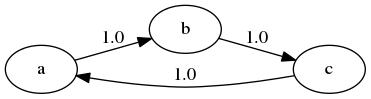
For example, the stochastic matrix associated with the transition probabilities below is periodic because, for example, state \(a\) has period 2
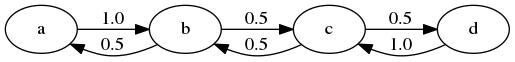
We can confirm that the stochastic matrix is periodic as follows
P = zeros(4, 4);
P[1, 2] = 1;
P[2, 1] = P[2, 3] = 0.5;
P[3, 2] = P[3, 4] = 0.5;
P[4, 3] = 1;
period(P)
2
is_aperiodic(P)
false
24.6. Stationary Distributions#
As seen in (24.5), we can shift probabilities forward one unit of time via postmultiplication by \(P\).
Some distributions are invariant under this updating process — for example,
P = [0.4 0.6; 0.2 0.8];
psi = [0.25, 0.75];
psi' * P
1×2 adjoint(::Vector{Float64}) with eltype Float64:
 0.25  0.75
Such distributions are called stationary, or invariant.
Formally, a distribution \(\psi^*\) on \(S\) is called stationary for \(P\) if \(\psi^* = \psi^* P\).
From this equality we immediately get \(\psi^* = \psi^* P^t\) for all \(t\).
This tells us an important fact: If the distribution of \(X_0\) is a stationary distribution, then \(X_t\) will have this same distribution for all \(t\).
Hence stationary distributions have a natural interpretation as stochastic steady states — we’ll discuss this more in just a moment.
Mathematically, a stationary distribution is a fixed point of \(P\) when \(P\) is thought of as the map \(\psi \mapsto \psi P\) from (row) vectors to (row) vectors.
Theorem. Every stochastic matrix \(P\) has at least one stationary distribution.
(We are assuming here that the state space \(S\) is finite; if not more assumptions are required)
For a proof of this result you can apply Brouwer’s fixed point theorem, or see EDTC, theorem 4.3.5.
There may in fact be many stationary distributions corresponding to a given stochastic matrix \(P\).
For example, if \(P\) is the identity matrix, then all distributions are stationary.
Since stationary distributions are long run equilibria, to get uniqueness we require that initial conditions are not infinitely persistent.
Infinite persistence of initial conditions occurs if certain regions of the state space cannot be accessed from other regions, which is the opposite of irreducibility.
This gives some intuition for the following fundamental theorem.
Theorem. If \(P\) is both aperiodic and irreducible, then
\(P\) has exactly one stationary distribution \(\psi^*\).
For any initial distribution \(\psi_0\), we have \(\| \psi_0 P^t - \psi^* \| \to 0\) as \(t \to \infty\).
For a proof, see, for example, theorem 5.2 of [Haggstrom02].
(Note that part 1 of the theorem requires only irreducibility, whereas part 2 requires both irreducibility and aperiodicity)
A stochastic matrix satisfying the conditions of the theorem is sometimes called uniformly ergodic.
One easy sufficient condition for aperiodicity and irreducibility is that every element of \(P\) is strictly positive
Try to convince yourself of this
24.6.1. Example#
Recall our model of employment / unemployment dynamics for a given worker discussed above.
Assuming \(\alpha \in (0,1)\) and \(\beta \in (0,1)\), the uniform ergodicity condition is satisfied.
Let \(\psi^* = (p, 1-p)\) be the stationary distribution, so that \(p\) corresponds to unemployment (state 1).
Using \(\psi^* = \psi^* P\) and a bit of algebra yields
This is, in some sense, a steady state probability of unemployment — more on interpretation below.
Not surprisingly it tends to zero as \(\beta \to 0\), and to one as \(\alpha \to 0\).
24.6.2. Calculating Stationary Distributions#
As discussed above, a given Markov matrix \(P\) can have many stationary distributions.
That is, there can be many row vectors \(\psi\) such that \(\psi = \psi P\).
In fact if \(P\) has two distinct stationary distributions \(\psi_1, \psi_2\) then it has infinitely many, since in this case, as you can verify,
is a stationary distribution for \(P\) for any \(\lambda \in [0, 1]\).
If we restrict attention to the case where only one stationary distribution exists, one option for finding it is to try to solve the linear system \(\psi (I_n - P) = 0\) for \(\psi\), where \(I_n\) is the \(n \times n\) identity.
But the zero vector solves this equation.
Hence we need to impose the restriction that the solution must be a probability distribution.
The helper stationary_distributions we wrote in Helper functions selects the eigenvectors of \(P'\) with unit eigenvalue and normalizes each to sum to one (use the first element if the stationary distribution is unique).
P = [0.4 0.6;
     0.2 0.8];
@show length(stationary_distributions(P))
stationary_distributions(P)[1]
length(stationary_distributions(P)) = 1
2-element Vector{Float64}:
 0.25
 0.7500000000000001
The stationary distribution is unique.
24.6.3. Convergence to Stationarity#
Part 2 of the Markov chain convergence theorem stated above tells us that the distribution of \(X_t\) converges to the stationary distribution regardless of where we start off.
This adds considerable weight to our interpretation of \(\psi^*\) as a stochastic steady state.
The convergence in the theorem is illustrated in the next figure
P = [0.971 0.029 0.000;
     0.145 0.778 0.077;
     0.000 0.508 0.492]

psi = [0.0 0.2 0.8] # initial distribution

t = 20
x_vals = zeros(t)
y_vals = similar(x_vals)
z_vals = similar(x_vals)
colors = [repeat([:red], 20); :black]

for i in 1:t
    x_vals[i] = psi[1]
    y_vals[i] = psi[2]
    z_vals[i] = psi[3]
    psi = psi * P # update distribution
end

psi_star = stationary_distributions(P)[1]
x_star, y_star, z_star = psi_star # unpack the stationary dist
plt = scatter([x_vals; x_star], [y_vals; y_star], [z_vals; z_star], color = colors,
              gridalpha = 0.5, legend = :none)
plot!(plt, camera = (45, 45))

Here
\(P\) is the stochastic matrix for recession and growth considered above
The highest red dot is an arbitrarily chosen initial probability distribution \(\psi\), represented as a vector in \(\mathbb R^3\)
The other red dots are the distributions \(\psi P^t\) for \(t = 1, 2, \ldots\)
The black dot is \(\psi^*\)
The code for the figure can be found here — you might like to try experimenting with different initial conditions.
24.7. Ergodicity#
Under irreducibility, yet another important result obtains: For all \(x \in S\),
Here
\(\mathbf{1}\{X_t = x\} = 1\) if \(X_t = x\) and zero otherwise
convergence is with probability one
the result does not depend on the distribution (or value) of \(X_0\)
The result tells us that the fraction of time the chain spends at state \(x\) converges to \(\psi^*(x)\) as time goes to infinity.
This gives us another way to interpret the stationary distribution — provided that the convergence result in (24.8) is valid.
The convergence in (24.8) is a special case of a law of large numbers result for Markov chains — see EDTC, section 4.3.4 for some additional information.
24.7.1. Example#
Recall our cross-sectional interpretation of the employment / unemployment model discussed above.
Assume that \(\alpha \in (0,1)\) and \(\beta \in (0,1)\), so that irreducibility and aperiodicity both hold.
We saw that the stationary distribution is \((p, 1-p)\), where
In the cross-sectional interpretation, this is the fraction of people unemployed.
In view of our latest (ergodicity) result, it is also the fraction of time that a worker can expect to spend unemployed.
Thus, in the long-run, cross-sectional averages for a population and time-series averages for a given person coincide.
This is one interpretation of the notion of ergodicity.
24.8. Computing Expectations#
We are interested in computing expectations of the form
and conditional expectations such as
where
\(\{X_t\}\) is a Markov chain generated by \(n \times n\) stochastic matrix \(P\)
\(h\) is a given function, which, in expressions involving matrix algebra, we’ll think of as the column vector
The unconditional expectation (24.9) is easy: We just sum over the distribution of \(X_t\) to get
Here \(\psi\) is the distribution of \(X_0\).
Since \(\psi\) and hence \(\psi P^t\) are row vectors, we can also write this as
For the conditional expectation (24.10), we need to sum over the conditional distribution of \(X_{t + k}\) given \(X_t = x\).
We already know that this is \(P^k(x, \cdot)\), so
The vector \(P^k h\) stores the conditional expectation \(\mathbb E [ h(X_{t + k}) \mid X_t = x]\) over all \(x\).
24.8.1. Expectations of Geometric Sums#
Sometimes we also want to compute expectations of a geometric sum, such as \(\sum_t \beta^t h(X_t)\).
In view of the preceding discussion, this is
where
Premultiplication by \((I - \beta P)^{-1}\) amounts to “applying the resolvent operator”.
24.9. Exercises#
24.9.1. Exercise 1#
According to the discussion above, if a worker’s employment dynamics obey the stochastic matrix
with \(\alpha \in (0,1)\) and \(\beta \in (0,1)\), then, in the long-run, the fraction of time spent unemployed will be
In other words, if \(\{X_t\}\) represents the Markov chain for employment, then \(\bar X_m \to p\) as \(m \to \infty\), where
Your exercise is to illustrate this convergence.
First,
generate one simulated time series \(\{X_t\}\) of length 10,000, starting at \(X_0 = 1\)
plot \(\bar X_m - p\) against \(m\), where \(p\) is as defined above
Second, repeat the first step, but this time taking \(X_0 = 2\).
In both cases, set \(\alpha = \beta = 0.1\).
The result should look something like the following — modulo randomness, of course
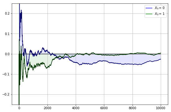
(You don’t need to add the fancy touches to the graph — see the solution if you’re interested)
24.9.2. Exercise 2#
A topic of interest for economics and many other disciplines is ranking.
Let’s now consider one of the most practical and important ranking problems — the rank assigned to web pages by search engines.
(Although the problem is motivated from outside of economics, there is in fact a deep connection between search ranking systems and prices in certain competitive equilibria — see [DLP13])
To understand the issue, consider the set of results returned by a query to a web search engine.
For the user, it is desirable to
receive a large set of accurate matches
have the matches returned in order, where the order corresponds to some measure of “importance”
Ranking according to a measure of importance is the problem we now consider.
The methodology developed to solve this problem by Google founders Larry Page and Sergey Brin is known as PageRank.
To illustrate the idea, consider the following diagram
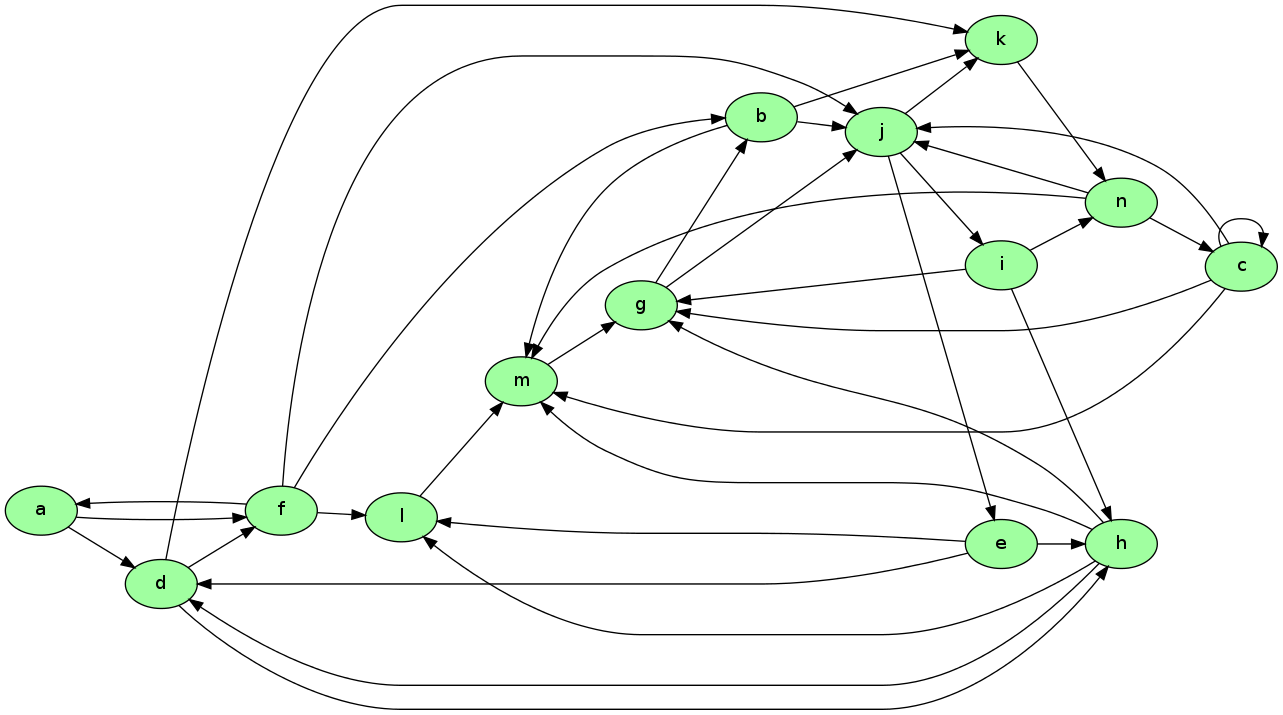
Imagine that this is a miniature version of the WWW, with
each node representing a web page
each arrow representing the existence of a link from one page to another
Now let’s think about which pages are likely to be important, in the sense of being valuable to a search engine user.
One possible criterion for importance of a page is the number of inbound links — an indication of popularity.
By this measure, m and j are the most important pages, with 5 inbound links each.
However, what if the pages linking to m, say, are not themselves important?
Thinking this way, it seems appropriate to weight the inbound nodes by relative importance.
The PageRank algorithm does precisely this.
A slightly simplified presentation that captures the basic idea is as follows.
Letting \(j\) be (the integer index of) a typical page and \(r_j\) be its ranking, we set
where
\(\ell_i\) is the total number of outbound links from \(i\)
\(L_j\) is the set of all pages \(i\) such that \(i\) has a link to \(j\)
This is a measure of the number of inbound links, weighted by their own ranking (and normalized by \(1 / \ell_i\)).
There is, however, another interpretation, and it brings us back to Markov chains.
Let \(P\) be the matrix given by \(P(i, j) = \mathbf 1\{i \to j\} / \ell_i\) where \(\mathbf 1\{i \to j\} = 1\) if \(i\) has a link to \(j\) and zero otherwise.
The matrix \(P\) is a stochastic matrix provided that each page has at least one link.
With this definition of \(P\) we have
Writing \(r\) for the row vector of rankings, this becomes \(r = r P\).
Hence \(r\) is the stationary distribution of the stochastic matrix \(P\).
Let’s think of \(P(i, j)\) as the probability of “moving” from page \(i\) to page \(j\).
The value \(P(i, j)\) has the interpretation
\(P(i, j) = 1/k\) if \(i\) has \(k\) outbound links, and \(j\) is one of them
\(P(i, j) = 0\) if \(i\) has no direct link to \(j\)
Thus, motion from page to page is that of a web surfer who moves from one page to another by randomly clicking on one of the links on that page.
Here “random” means that each link is selected with equal probability.
Since \(r\) is the stationary distribution of \(P\), assuming that the uniform ergodicity condition is valid, we can interpret \(r_j\) as the fraction of time that a (very persistent) random surfer spends at page \(j\).
Your exercise is to apply this ranking algorithm to the graph pictured above, and return the list of pages ordered by rank.
When you solve for the ranking, you will find that the highest ranked node is in fact g, while the lowest is a.
24.10. Solutions#
24.10.1. Exercise 1#
Compute the fraction of time that the worker spends unemployed, and compare it to the stationary probability.
alpha = 0.1 # probability of getting hired
beta = 0.1 # probability of getting fired
N = 10_000
p_bar = beta / (alpha + beta) # steady-state probabilities
P = [1-alpha alpha
     beta 1-beta] # stochastic matrix
labels = ["start unemployed", "start employed"]
y_vals = Array{Vector}(undef, 2) # sample paths holder

for x0 in 1:2
    X = mc_sample_path(P; init = x0, sample_size = N) # generate the sample path
    X_bar = cumsum(X .== 1) ./ (1:N) # compute state fraction. ./ required for precedence
    y_vals[x0] = X_bar .- p_bar # plot divergence from steady state
end

plot(y_vals, color = [:blue :green], fillrange = 0, fillalpha = 0.1,
     ylims = (-0.25, 0.25), label = reshape(labels, 1, length(labels)))

24.10.2. Exercise 2#
web_graph_data = Dict(
    'a' => ['d','f'],
    'b' => ['j','k','m'],
    'c' => ['c','g','j','m'],
    'd' => ['f','h','k'],
    'e' => ['d','h','l'],
    'f' => ['a','b','j','l'],
    'g' => ['b','j'],
    'h' => ['d','g','l','m'],
    'i' => ['g','h','n'],
    'j' => ['e','i','k'],
    'k' => ['n'],
    'l' => ['m'],
    'm' => ['g'],
    'n' => ['c','j','m']
)

# 1. Sort nodes to ensure consistent matrix indexing (a=1, b=2, etc.)
nodes = sort(collect(keys(web_graph_data)))
index_map = Dict(c => i for (i, c) in enumerate(nodes))
n = length(nodes)

# 2. Build Stochastic Matrix P directly
P = zeros(n, n)

for (from_node, targets) in web_graph_data
    i = index_map[from_node]
    k = length(targets) # number of outbound links

    # Assign equal probability to each outbound link
    for to_node in targets
        j = index_map[to_node]
        P[i, j] = 1.0 / k
    end
end
Next we find the ranking by computing the stationary distribution and then sorting the pages accordingly.
r = stationary_distributions(P)[1] # stationary distribution

# Use 'nodes' which matches the ordering of 'r'
ranked_pages = Dict(zip(nodes, r))

# Print solution.  Sort the (node, r) by the rank value descending
for (node, rank) in sort(collect(ranked_pages), by = x -> x[2], rev = true)
    println("'$node' => $rank")
end
'g' => 0.16070778858515058
'j' => 0.15936158342833584
'm' => 0.1195151235840589
'n' => 0.10876973827831274
'k' => 0.09106289567516433
'b' => 0.08326460814514758
'i' => 0.053120527809445345
'e' => 0.05312052780944534
'c' => 0.04834210590147239
'h' => 0.04560118369030011
'l' => 0.032017852378295714
'd' => 0.03056249545200956
'f' => 0.01164285541028925
'a' => 0.0029107138525722425