10. Optimization and Nonlinear Solvers#
Contents
10.1. Overview#
In this lecture we introduce a few of the Julia libraries for solving optimization problems, systems of equations, and finding fixed points.
See auto-differentiation for more on calculating gradients and Jacobians for these types of algorithms.
using Pkg; pkgs = ["BenchmarkTools", "Enzyme", "FixedPointAcceleration", "ForwardDiff", "NLsolve", "NonlinearSolve", "Optim", "Optimization", "OptimizationOptimJL", "Roots", "StaticArrays"]; all(haskey.(Ref(Pkg.project().dependencies), pkgs)) || Pkg.add(pkgs)
using LinearAlgebra, Statistics, BenchmarkTools
using ForwardDiff, Optim, Roots, NLsolve
using FixedPointAcceleration, NonlinearSolve
using Optimization, OptimizationOptimJL, ForwardDiff, Enzyme
using Optim: converged, maximum, maximizer, minimizer, iterations #some extra functions
using StaticArrays
10.2. Optimization#
There are a large number of packages intended to be used for optimization in Julia.
Part of the reason for the diversity of options is that Julia makes it possible to efficiently implement a large number of variations on optimization routines.
The other reason is that different types of optimization problems require different algorithms.
10.2.1. Optim.jl#
A good pure-Julia solution for the (unconstrained or box-bounded) optimization of univariate and multivariate functions is the Optim.jl package.
By default, the algorithms in Optim.jl target minimization rather than
maximization, so if a function is called optimize it will mean minimization.
10.2.1.1. Univariate Functions on Bounded Intervals#
Univariate optimization defaults to a robust hybrid optimization routine called Brent’s method.
using Optim: converged, maximum, maximizer, minimizer, iterations #some extra functions

result = optimize(x -> x^2, -2.0, 1.0)
Results of Optimization Algorithm
 * Status: success
 * Algorithm: Brent's Method
 * Search Interval: [-2.000000, 1.000000]
 * Minimizer: 0.000000e+00
 * Minimum: 0.000000e+00
 * Iterations: 5
 * Convergence: max(|x - x_upper|, |x - x_lower|) <= 2*(1.5e-08*|x|+2.2e-16): true
 * Objective Function Calls: 6
Always check if the results converged, and throw errors otherwise
converged(result) ||
    error("Failed to converge in $(iterations(result)) iterations")
xmin = result.minimizer
result.minimum
0.0
The first line is a logical OR between converged(result) and error("...").
If the convergence check passes, the logical sentence is true, and it will proceed to the next line; if not, it will throw the error.
10.2.1.2. Unconstrained Multivariate Optimization#
There are a variety of algorithms and options for multivariate optimization.
From the documentation, the simplest version is
f(x) = (1.0 - x[1])^2 + 100.0 * (x[2] - x[1]^2)^2
x_iv = [0.0, 0.0]
results = optimize(f, x_iv) # i.e. optimize(f, x_iv, NelderMead())
 * Status: success

 * Candidate solution
    Final objective value:     3.525527e-09

 * Found with
    Algorithm:     Nelder-Mead

 * Convergence measures
    √(Σ(yᵢ-ȳ)²)/n ≤ 1.0e-08

 * Work counters
    Seconds run:   0  (vs limit Inf)
    Iterations:    60
    f(x) calls:    117
The default algorithm is NelderMead, which is derivative-free and hence requires many function evaluations.
To change the algorithm type to L-BFGS
results = optimize(f, x_iv, LBFGS())
println("minimum = $(results.minimum) with argmin = $(results.minimizer) in " *
        "$(results.iterations) iterations")
minimum = 5.3784046148998115e-17 with argmin = [0.9999999926662393, 0.9999999853324786] in 24 iterations
Note that this has fewer iterations.
As no derivative was given, it used finite differences to approximate the gradient of f(x).
However, since most of the algorithms require derivatives, you will often want to use automatic differentiation or pass analytical gradients if possible.
f(x) = (1.0 - x[1])^2 + 100.0 * (x[2] - x[1]^2)^2
x_iv = [0.0, 0.0]
results = optimize(f, x_iv, LBFGS(), autodiff = :forward) # i.e. use ForwardDiff.jl
println("minimum = $(results.minimum) with argmin = $(results.minimizer) in " *
        "$(results.iterations) iterations")
minimum = 5.191703158437428e-27 with argmin = [0.999999999999928, 0.9999999999998559] in 24 iterations
Note that we did not need to use ForwardDiff.jl directly, as long as our f(x) function was written to be generic (see the generic programming lecture ).
Alternatively, with an analytical gradient
f(x) = (1.0 - x[1])^2 + 100.0 * (x[2] - x[1]^2)^2
x_iv = [0.0, 0.0]
function g!(G, x)
    G[1] = -2.0 * (1.0 - x[1]) - 400.0 * (x[2] - x[1]^2) * x[1]
    G[2] = 200.0 * (x[2] - x[1]^2)
end

results = optimize(f, g!, x_iv, LBFGS()) # or ConjugateGradient()
println("minimum = $(results.minimum) with argmin = $(results.minimizer) in " *
        "$(results.iterations) iterations")
minimum = 5.191703158437428e-27 with argmin = [0.999999999999928, 0.9999999999998559] in 24 iterations
For derivative-free methods, you can change the algorithm – and have no need to provide a gradient
f(x) = (1.0 - x[1])^2 + 100.0 * (x[2] - x[1]^2)^2
x_iv = [0.0, 0.0]
results = optimize(f, x_iv, SimulatedAnnealing()) # or ParticleSwarm() or NelderMead()
 * Status: failure (reached maximum number of iterations)

 * Candidate solution
    Final objective value:     1.595707e-03

 * Found with
    Algorithm:     Simulated Annealing

 * Convergence measures
    |x - x'|               = NaN ≰ 0.0e+00
    |x - x'|/|x'|          = NaN ≰ 0.0e+00
    |f(x) - f(x')|         = NaN ≰ 0.0e+00
    |f(x) - f(x')|/|f(x')| = NaN ≰ 0.0e+00
    |g(x)|                 = NaN ≰ 1.0e-08

 * Work counters
    Seconds run:   0  (vs limit Inf)
    Iterations:    1000
    f(x) calls:    1001
However, you will note that this did not converge, as stochastic methods typically require many more iterations as a tradeoff for their global convergence properties.
See the maximum likelihood example and the accompanying Jupyter notebook.
10.2.2. JuMP.jl#
The JuMP.jl package is an ambitious implementation of a modelling language for optimization problems in Julia.
In that sense, it is more like an AMPL (or Pyomo) built on top of the Julia language with macros, and able to use a variety of different commercial and open-source solvers.
If you have a linear, quadratic, conic, mixed-integer linear, etc. problem then this will likely be the ideal “meta-package” for calling various solvers.
For nonlinear problems, the modelling language may make things difficult for complicated functions (as it is not designed to be used as a general-purpose nonlinear optimizer).
See the quick start guide for more details on all of the options.
The following is an example of calling a linear objective with a nonlinear constraint (provided by an external function).
Here Ipopt stands for Interior Point OPTimizer, a nonlinear solver in Julia
using JuMP, Ipopt
# solve
# max( x[1] + x[2] )
# st sqrt(x[1]^2 + x[2]^2) <= 1

function squareroot(x) # pretending we don't know sqrt()
    z = x # Initial starting point for Newton’s method
    while abs(z * z - x) > 1e-13
        z = z - (z * z - x) / (2z)
    end
    return z
end
m = Model(Ipopt.Optimizer)
# need to register user defined functions for AD
JuMP.register(m, :squareroot, 1, squareroot, autodiff = true)

@variable(m, x[1:2], start=0.5) # start is the initial condition
@objective(m, Max, sum(x))
@NLconstraint(m, squareroot(x[1]^2 + x[2]^2)<=1)
@show JuMP.optimize!(m)
And this is an example of a quadratic objective
# solve
# min (1-x)^2 + (100(y-x^2)^2)
# st x + y >= 10

using JuMP, Ipopt
m = Model(Ipopt.Optimizer) # settings for the solver
@variable(m, x, start=0.0)
@variable(m, y, start=0.0)

@NLobjective(m, Min, (1 - x)^2+100(y - x^2)^2)

JuMP.optimize!(m)
println("x = ", value(x), " y = ", value(y))

# adding a (linear) constraint
@constraint(m, x + y==10)
JuMP.optimize!(m)
println("x = ", value(x), " y = ", value(y))
10.2.3. BlackBoxOptim.jl#
Another package for doing global optimization without derivatives is BlackBoxOptim.jl.
An example for parallel execution of the objective is provided.
10.3. Optimization.jl Meta-Package#
The Optimization.jl package provides a common interface to a variety of optimization packages in Julia. As part of the SciML ecosystem, it is designed to work seamlessly with other SciML tools, and to provide differentiable optimization routines that can be used in conjunction with automatic differentiation packages.
Algorithms require loading additional packages for one of the supported optimizers, such as OptimizationOptimJL.jl, which wraps the Optim.jl package.
From the documentation:
rosenbrock(u, p) = (p[1] - u[1])^2 + p[2] * (u[2] - u[1]^2)^2
u0 = zeros(2)
p = [1.0, 100.0]
prob = OptimizationProblem(rosenbrock, u0, p)
sol = solve(prob, NelderMead())
sol
retcode: Success
u: 2-element Vector{Float64}:
 0.9999634355313174
 0.9999315506115275
The separation of the argument, u, and the parameters, p, is common in SciML and provides methods to cleanly handle parameterized problems.
Function wrappers also provide easy integration with automatic differentiation such as ForwardDiff.jl.
f_fd = OptimizationFunction(rosenbrock, Optimization.AutoForwardDiff())
prob = OptimizationProblem(f_fd, u0, p)
sol = solve(prob, BFGS())
retcode: Success
u: 2-element Vector{Float64}:
 0.9999999999373603
 0.99999999986862
Or with Enzyme.jl, which has slower compilation times but provides another AD backend
f_enzyme = OptimizationFunction(rosenbrock, Optimization.AutoEnzyme())
prob = OptimizationProblem(f_enzyme, u0, p)
sol = solve(prob, BFGS())
retcode: Success
u: 2-element Vector{Float64}:
 0.9999999999373603
 0.9999999998686199
Finally, the documentation for a variety of other examples and features, such as constrained optimization.
10.4. NonlinearSolve.jl Meta-Package#
Within the SciML ecosystem, the NonlinearSolve.jl package provides a unified interface for solving nonlinear systems of equations. It builds on top of other SciML packages and offers advanced features such as automatic differentiation, various solver algorithms, and support for large-scale problems. Furthermore, as with Optimization.jl, it has convenient integration with automatic differentiation (as well as implementing AD for the solver itself, with respect to parameters).
In general, we suggest using this meta-package where possible as it provides a well-maintained interface amenable to switching out solvers in the future.
10.4.1. Basic Examples#
Here we adapt examples directly from the documentation.
First we can solve a system of equations as a closure over a constant c.
c = 2.0
f(u, p) = u .* u .- c # p ignored
u0 = [1.0, 1.0]
prob = NonlinearProblem(f, u0) # defaults to p = nothing
sol = solve(prob, NewtonRaphson())
retcode: Success
u: 2-element Vector{Float64}:
 1.4142135623730951
 1.4142135623730951
In this case, the p argument (which can hold parameters) is ignored, but needs to be present in SciML problems.
The NewtonRaphson() method is a built-in solver, and not an external package. We can access the results through sol.u and see other information such as the return code
@show sol.u
@show sol.retcode
sol.stats
sol.u = [1.4142135623730951, 1.4142135623730951]
sol.retcode =
SciMLBase.ReturnCode.Success
SciMLBase.NLStats
Number of function evaluations:                    7
Number of Jacobians created:                       6
Number of factorizations:                          0
Number of linear solves:                           5
Number of nonlinear solver iterations:             5
We can see further details on the algorithm itself, and see that it uses ForwardDiff.jl by default since NewtonRaphson() requires a Jacobian.
sol.alg
NewtonRaphson(
    descent = NewtonDescent(),
    autodiff = AutoForwardDiff(),
    vjp_autodiff = AutoEnzyme(
        mode = ReverseMode()
    ),
    jvp_autodiff = AutoForwardDiff(),
    concrete_jac = Val{false}()
)
You can see the performance of this algorithm in this context, which uses a large number of allocations relative to the simplicity of the problem.
@benchmark solve($prob, NewtonRaphson())
BenchmarkTools.Trial: 10000 samples with 1 evaluation per sample.
 Range (min … max):  16.200 μs … 92.086 μs  ┊ GC (min … max): 0.00% … 0.00%
 Time  (median):     16.701 μs              ┊ GC (median):    0.00%
 Time  (mean ± σ):   16.912 μs ±  1.407 μs  ┊ GC (mean ± σ):  0.00% ± 0.00%

    ▅█▆▄▂
  ▂▅█████▇▆▅▄▃▃▃▃▂▂▂▂▂▂▂▂▂▂▂▂▂▂▂▂▂▂▁▂▂▁▁▁▁▁▂▁▁▁▁▁▁▂▂▂▂▂▂▂▂▂▂▂ ▃
  16.2 μs         Histogram: frequency by time        22.1 μs <

 Memory estimate: 7.06 KiB, allocs estimate: 132.
10.4.2. Using Parameters and Inplace Functions#
SciML interfaces prefer to cleanly separate a function argument and a parameter argument, which makes it easier to handle parameterized problems and ensure flexible code.
To use this, we rewrite our example above to use the previously ignored parameter p.
f(u, p) = u .* u .- p
u0 = [1.0, 1.0]
p = 2.0
prob = NonlinearProblem(f, u0, p) # pass the `p`
NonlinearProblem with uType Vector{Float64}. In-place: false
u0: 2-element Vector{Float64}:
 1.0
 1.0
Note that the prob shows In-place: true.
Benchmarking this version.
@btime solve($prob, NewtonRaphson())
9.689 μs
(99 allocations: 6.06 KiB)
retcode: Success
u: 2-element Vector{Float64}:
 1.4142135623730951
 1.4142135623730951
This may or may not have better performance than the previous version which used the closure.
Regardless, it will still have many allocations, which can be a significant fraction of the runtime for problems small or large.
To support this, the SciML ecosystem has a bias towards in-place functions. Here we add another version of the function f!(du, u, p) to be in-place, modifying the first argument, which the solver detects.
function f!(du, u, p)
    du .= u .* u .- p
end
prob = NonlinearProblem(f!, u0, p)
@btime solve($prob, NewtonRaphson())
8.703 μs
(65 allocations: 4.44 KiB)
retcode: Success
u: 2-element Vector{Float64}:
 1.4142135623730951
 1.4142135623730951
Note the decrease in allocations, and possibly time depending on your system.
10.4.3. Patterns for Parameters#
The p argument can be anything, including named tuples, vectors, or a single value as above.
A common pattern appropriate for more complicated code is to use a named tuple packing and unpacking.
function f_nt(u, p)
    (; c) = p # unpack any arguments in the named tuple
    return u .* u .- c
end

p_nt = (c = 2.0,) # named tuple
prob_nt = NonlinearProblem(f_nt, u0, p_nt)
@btime solve($prob_nt, NewtonRaphson())
9.682 μs
(99 allocations: 6.06 KiB)
retcode: Success
u: 2-element Vector{Float64}:
 1.4142135623730951
 1.4142135623730951
10.4.4. Small Systems#
For small systems, the solver is able to use StaticArrays.jl which can further improve performance. These fixed-size arrays require using the out-of-place formulation, but otherwise require no special handling.
using StaticArrays
f_SA(u, p) = SA[u[1] * u[1] - p, u[2] * u[2] - p] # rewrote without broadcasting
u0_static = SA[1.0, 1.0] # static array
prob = NonlinearProblem(f_SA, u0_static, p)
NonlinearProblem with uType SVector{2, Float64}. In-place: false
u0: 2-element SVector{2, Float64} with indices SOneTo(2):
 1.0
 1.0
Note that the problem shows that this is In-place: false and operates on the SVector{2, Float64} type.
Next we can benchmark this version, where we can use a simpler non-allocating solver designed for small systems, SimpleNewtonRaphson(). See the docs for more details on solvers optimized for non-allocating algorithms.
@btime solve($prob, SimpleNewtonRaphson())
49.624 ns
(0 allocations: 0 bytes)
retcode: Success
u: 2-element SVector{2, Float64} with indices SOneTo(2):
 1.414213562373095
 1.414213562373095
Depending on your system, you may find this is 100 to 1000x faster than the original version using closures and allocations.
Note
In principle it should be equivalent to use our previous f instead of f_SA, but depending on package and compiler versions it may not achieve the full 0 allocations. Regardless, try the generic function first before porting over to a new function. The SimpleNewtonRaphson() function is also specialized to avoid any internal allocations for small systems, but you will even see some benefits with NewtonRaphson().
10.4.5. Using Other Solvers#
While it has some pre-built solvers, as we used above, it is primarily intended as a meta-package. To use one of the many external solver packages you simply need to ensure the package is in your Project file and then include it.
For example, we can use the Anderson Acceleration in FixedPointAcceleration.jl’s wrapper
using FixedPointAcceleration
prob = NonlinearProblem(f, u0, p)
@btime solve($prob, FixedPointAccelerationJL())
@btime solve($prob, FixedPointAccelerationJL(; algorithm = :Simple))
48.319 μs
 (862 allocations: 323.65 KiB)
  2.101 ms
(21324 allocations: 16.03 MiB)
retcode: Failure
u: 2-element Vector{Float64}:
 1.0
 1.0
The default algorithm in this case is :Anderson, but we can also use :Simple fixed-point iteration.
In this case, the fixed-point iteration algorithm is slower than the gradient-based Newton-Raphson, but shows the flexibility in cases where gradients are not available.
Note
While there is a NLsolve.jl wrapper, it seems to have a less robust implementation of Anderson than some of the other packages.
10.4.6. Bracketing Solvers and Rootfinding Problems#
The NonlinearProblem type is intended for algorithms which use an initial condition (and may or may not use derivatives).
For some one-dimensional problems it is more convenient to use one of the bracketing methods
For example, from the documentation,
f_bracketed(u, p) = u * u - p
uspan = (1.0, 2.0) # brackets
p = 2.0
prob = IntervalNonlinearProblem(f_bracketed, uspan, p)
sol = solve(prob)
retcode: Success
u: 1.414213562373095
In general, this should be preferred to using the Roots.jl package below, as it may provide a more consistent interface.
10.5. Systems of Equations and Fixed Points#
Julia has a variety of packages you can directly use for solving systems of equations and finding fixed points. Many of these packages can also be used as backends for the NonlinearSolve.jl meta-package described above.
10.5.1. Roots.jl#
A root of a real function \(f\) on \([a,b]\) is an \(x \in [a, b]\) such that \(f(x)=0\).
For example, if we plot the function
with \(x \in [0,1]\) we get
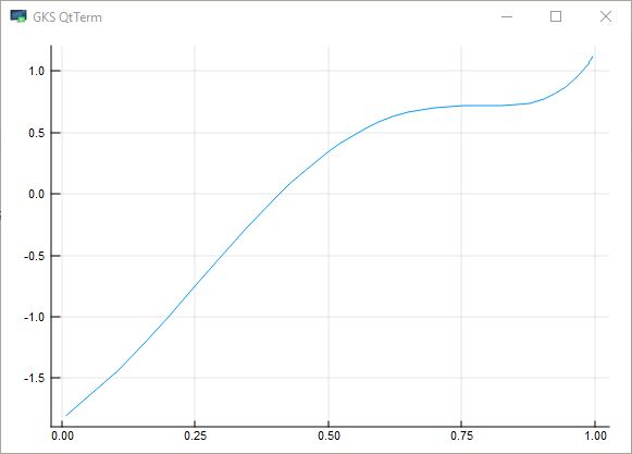
The unique root is approximately 0.408.
The Roots.jl package offers fzero() to find roots
using Roots
f(x) = sin(4 * (x - 1 / 4)) + x + x^20 - 1
fzero(f, 0, 1)
0.40829350427936706
10.5.2. NLsolve.jl#
The NLsolve.jl package provides functions to solve for multivariate systems of equations and fixed points.
From the documentation, to solve for a system of equations without providing a Jacobian
using NLsolve

f(x) = [(x[1] + 3) * (x[2]^3 - 7) + 18
        sin(x[2] * exp(x[1]) - 1)] # returns an array

results = nlsolve(f, [0.1; 1.2])
Results of Nonlinear Solver Algorithm
 * Algorithm: Trust-region with dogleg and autoscaling
 * Starting Point: [0.1, 1.2]
 * Zero: [-7.775548712324193e-17, 0.9999999999999999]
 * Inf-norm of residuals: 0.000000
 * Iterations: 4
 * Convergence: true
   * |x - x'| < 0.0e+00: false
   * |f(x)| < 1.0e-08: true
 * Function Calls (f): 5
 * Jacobian Calls (df/dx): 5
In the above case, the algorithm used finite differences to calculate the Jacobian.
Alternatively, if f(x) is written generically, you can use auto-differentiation with a single setting.
results = nlsolve(f, [0.1; 1.2], autodiff = :forward)

println("converged=$(NLsolve.converged(results)) at root=$(results.zero) in " *
        "$(results.iterations) iterations and $(results.f_calls) function calls")
converged=true at root=[-3.487552479724522e-16, 1.0000000000000002] in 4 iterations and 5 function calls
Providing a function which operates inplace (i.e., modifies an argument) may help performance for large systems of equations (and hurt it for small ones).
function f!(F, x) # modifies the first argument
    F[1] = (x[1] + 3) * (x[2]^3 - 7) + 18
    F[2] = sin(x[2] * exp(x[1]) - 1)
end

results = nlsolve(f!, [0.1; 1.2], autodiff = :forward)

println("converged=$(NLsolve.converged(results)) at root=$(results.zero) in " *
        "$(results.iterations) iterations and $(results.f_calls) function calls")
converged=true at root=[-3.487552479724522e-16, 1.0000000000000002] in 4 iterations and 5 function calls