1. Setting up Your Julia Environment#
Contents
1.1. Overview#
In this lecture we will cover how to get up and running with Julia.
While there are alternative ways to access Julia (e.g. if you have a JupyterHub provided by your university), this section assumes you will install it to your local desktop.
It is not strictly required for running the lectures, but we will strongly encourage installing and using Visual Studio Code (VS Code).
We will use it as our primary editor starting in the tools lecture.
1.2. TL;DR#
Julia and the lecture notebooks can be installed without Jupyter or Python:
Install Git
Install VS Code
Install Julia following the Juliaup instructions
Windows:
winget install julia -s msstorein a terminalLinux/Mac:
curl -fsSL https://install.julialang.org | shin a terminal
Install the VS Code Julia extension
In VS Code, open the command palette with
<Ctrl+Shift+P>and type> Git: Cloneto clone the repositoryhttps://github.com/quantecon/lecture-julia.notebooksin a new windowStart a Julia REPL in the integrated terminal with
> Julia: Start REPLfrom the command palette, then enter package mode with]and then typeinstantiate.
That process will take several minutes to download and compile all of the packages used in the lectures.
Open any of the
.ipynbfiles in VS Code and select theJuliachannel (i.e., not the Jupyter channels if you have them installed) when prompted to run the notebooks directly within VS Code
At that point, you can directly move to the julia by example lecture.
1.3. A Note on Jupyter#
Jupyter notebooks are an alternative way to work with Julia, letting you mix code, formatted text, and output in a single document. However, the recommended workflow for these lectures is VS Code (see Setting up Git and VS Code). If you prefer standalone Jupyter Lab, see the installation instructions below.
These lectures assume some prior programming experience (variables, loops, conditionals). The Julia documentation is a good starting point for newcomers.
1.4. Desktop Installation of Julia and Jupyter#
Note
This section is only needed if you want the standalone Jupyter Lab workflow. If you plan to use VS Code (recommended) or Google Colab, you can skip to Setting up Git and VS Code.
1.4.1. Installing Jupyter#
Anaconda provides an easy way to install Jupyter, Python, and many data science tools.
Download the binary (https://www.anaconda.com/download/) and follow the installation instructions for your platform.
If given the option, let Conda add Python to your PATH environment variables.
Note
There is direct support for Jupyter notebooks in VS Code with no Python installation. See VS Code Julia Kernel.
1.4.2. Install Julia#
Note
The “official” installation for Julia is now Juliaup, which makes it easier to upgrade and manage concurrent Julia versions. See here for a list of commands, such as juliaup update to upgrade to the latest available Julia version.
Troubleshooting: On Mac/Linux, if you have permissions issues on the installation use sudo curl -fsSL https://install.julialang.org | sh. If there are still permissions issues, see here for further steps.
Download and install Julia following the Juliaup instructions
Windows:
winget install julia -s msstorein a terminalLinux/Mac:
curl -fsSL https://install.julialang.org | shin a terminalIf you have previously installed Julia manually, you will need to uninstall previous versions before switching to
juliaup
Open Julia, by either
Navigating to Julia through your menus or desktop icons (Windows, Mac), or
Opening a terminal and typing
julia
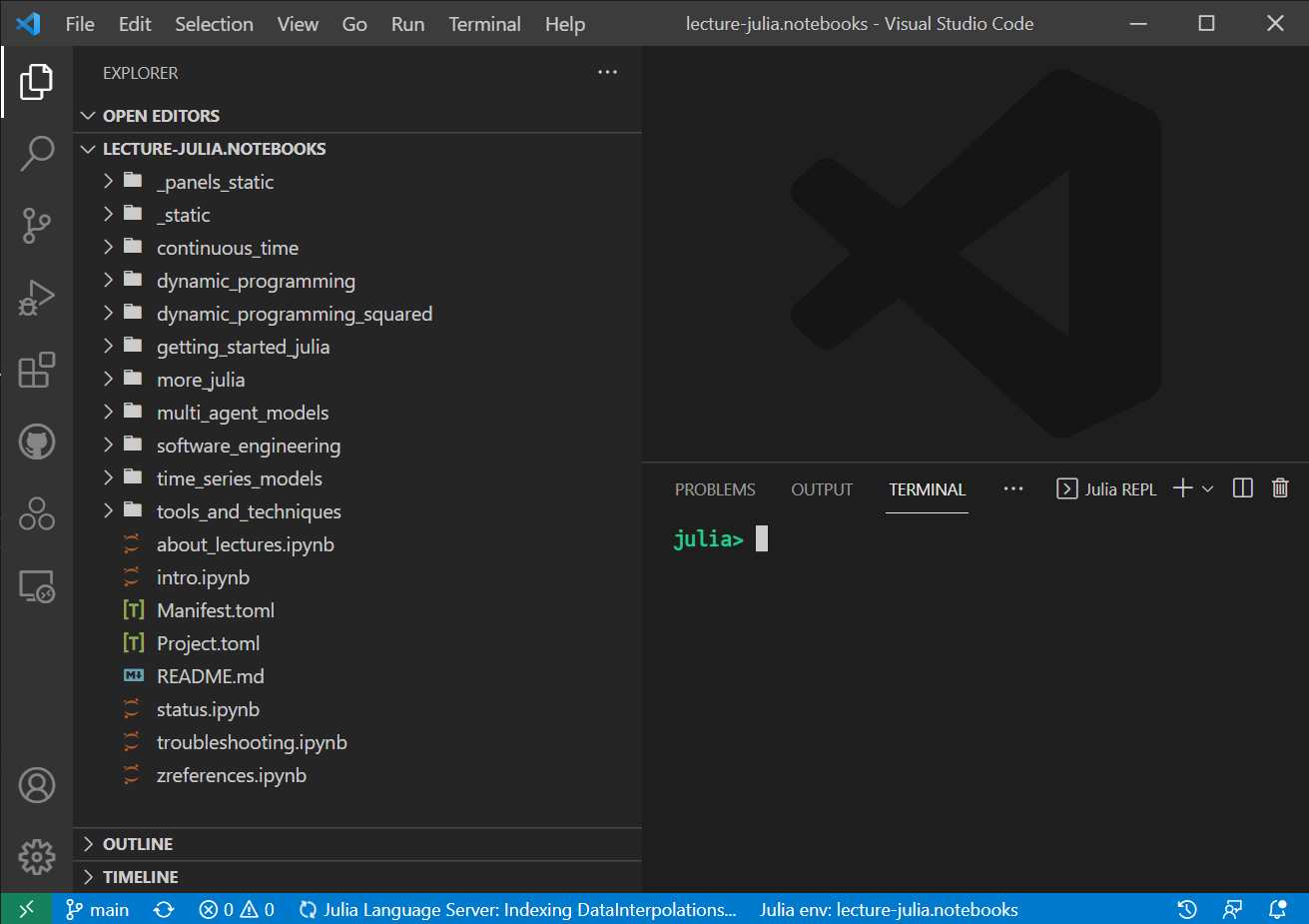
You should now be looking at something like this
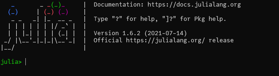
This is called the JULIA REPL (Read-Evaluate-Print-Loop), which we discuss more later.
In the Julia REPL, hit
]to enter package mode and then enter:add IJulia
This adds the
IJuliakernel which links Julia to Jupyter (i.e., allows your browser to run Julia code, manage Julia packages, etc.).Exit the package mode with backspace and then quit with
exit().
Note
As entering package mode is common in these notes, we will denote this with ] add IJulia, etc.
1.5. Setting up Git and VS Code#
First, install Git, the industry standard version-control tool, which lets you download files and their entire version history from a server (e.g. on GitHub) to your desktop. We cover Git in detail in the lectures on source code control and testing.
Install Git and accept the default arguments.
If you allow Git to add to your path, then you can run it with the
gitcommand, but we will frequently use the built-in VS Code features.
(Optional) Install VS Code for your platform and open it
On Windows, during install under
Select Additional Tasks, choose all options that begin withAdd "Open with Code" action. This lets you open VS Code from inside File Explorer folders directly.While optional, we find the experience with VS Code will be much easier and the transition to more advanced tools will be more seamless.
(Optional) Install the VS Code Julia extension
After installation of VS Code, you should be able to choose
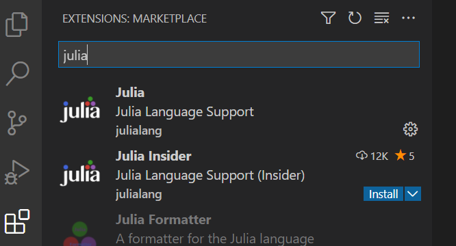
Installon the webpage of any extensions and it will open on your desktop.Otherwise: run VS Code and open the extensions with
<Ctrl+Shift+X>or selecting extensions in the left-hand side of the VS Code window. Then search forJuliain the Marketplace.
No further configuration should be required, but see here if you have issues.
The VS Code and the VS Code Julia extension will help us better manage environments during our initial setup, and will provide a seamless transition to the more advanced tools.
1.5.1. Command Palette on VS Code#
A key feature within VS Code is the Command Palette, which can be accessed with <Ctrl+Shift+P> or View > Command Palette... in the menus.

This is so common that in these notes we
denote opening the command palette and searching for a command with things like > Julia: Start REPL , etc.
1.6. Downloading the Notebooks#
Next, let’s install the QuantEcon lecture notes to our machine and run them (for more details on the tools we’ll use, see our lecture on version control).
Open the command palette with
<Ctrl+Shift+P>and type> Git: CloneFor the Repository URL, enter
https://github.com/quantecon/lecture-julia.notebooksChoose the location to clone when prompted
For example, on Windows a good choice is
c:\Users\YOURUSERNAME\Documents\GitHub. On Linux and macOS,~or~/GitHub.
Accept the option to open in a new window when prompted
Cloning without VS Code
Alternatively, you can clone from the command line:
Open a terminal and navigate to a convenient parent folder (see above for suggestions).
Run
git clone https://github.com/quantecon/lecture-julia.notebookscd lecture-julia.notebooksOpen the directory in VS Code with
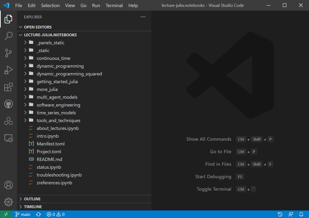
code ., or open it manually.
If you have opened this in VS Code, it should look something like
1.7. Installing Packages#
After you have the notebooks available, as described in the previous section, we can install the required packages for plotting, benchmarking, and statistics.
For this, we will use the integrated terminal in VS Code.
Recall that you can start this directly from the command palette with <Ctrl+Shift+P> then typing part of the > Julia: Start REPL command.
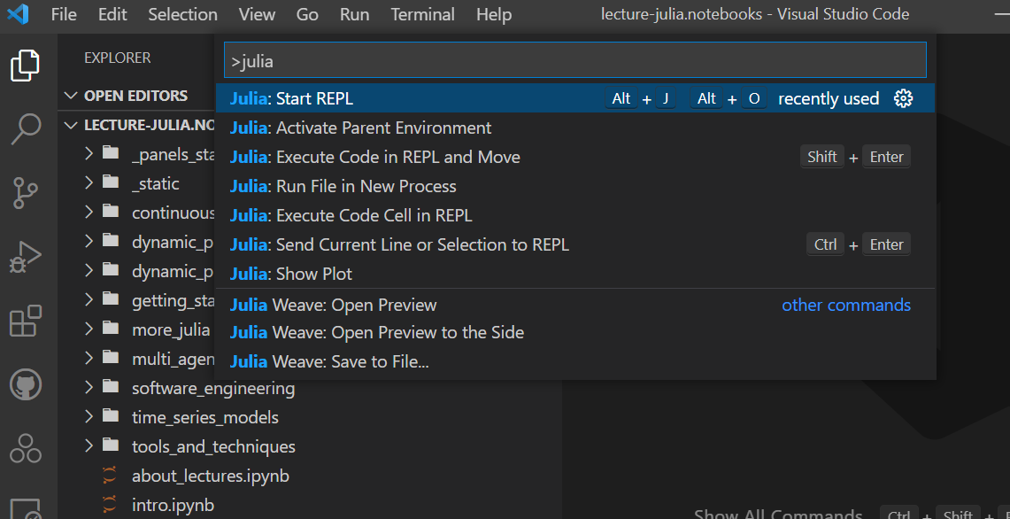
Start a REPL; it may do an initial compilation of packages in the background, but will then look something like
Next type
]to enter the package mode, which should indicate that the local project is activated by changing the cursor to(quantecon-notebooks-julia) pkg>.Type
instantiateto install all of the packages required for these notes.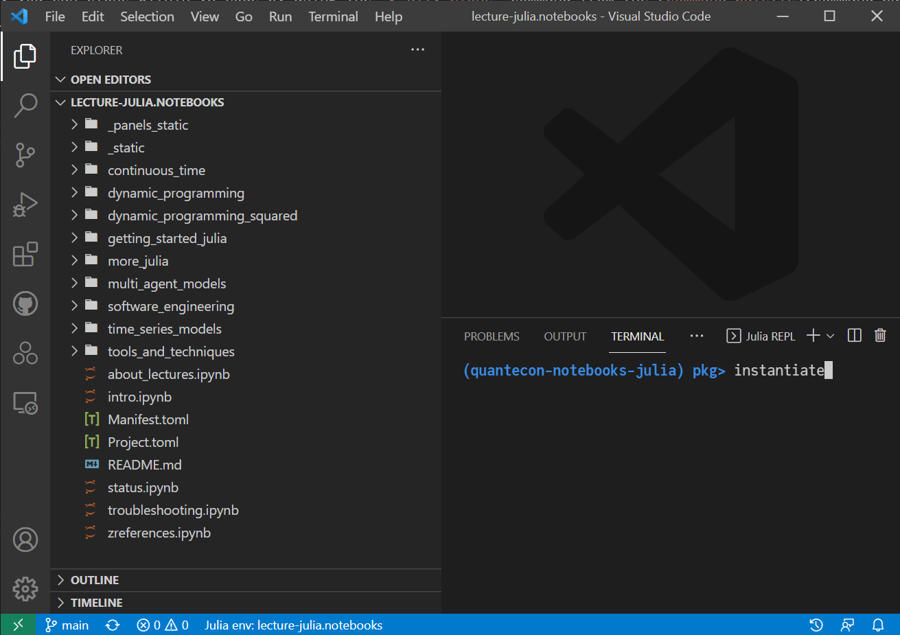
This process will take several minutes to download and compile all of the files used by the lectures.
Attention
If the package-mode cursor shows (@v1.x) pkg> instead of (quantecon-notebooks-julia) pkg>, type activate . to activate the local project.
Why use the integrated REPL?
The VS Code integrated REPL automatically sets thread count and activates the local project. If you use an external REPL, launch it with julia --project --threads auto. See here for details.
1.8. Running JupyterLab#
Note
This section is only needed for the standalone Jupyter Lab workflow. If you use VS Code, you can run notebooks directly — see VS Code Julia Kernel.
Open a terminal in the notebook directory and run:
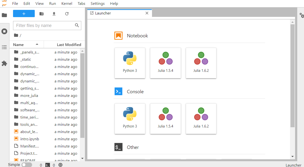
jupyter lab
This launches Jupyter with access to the current directory. A browser tab should open automatically; if not, follow the link shown in the terminal output.
1.9. Refreshing the Notebooks after Modification#
To revert notebooks to the latest version from the server:
In VS Code, open the “Source Control” pane (
<Ctrl+Shift+G>), right-click “Changes”, and selectDiscard All Changes.To pull the latest updates, use the
> Git: Pullcommand or click the sync arrow next to “main” in the status bar.
If the Project.toml or Manifest.toml files changed, re-enter package mode (]) and run instantiate to update packages.
We will explore these features in the source code control lecture.
1.10. Interacting with Julia#
If you are new to Jupyter notebooks, see the QuantEcon Python lecture for an introduction to the interface, including cells, execution, and keyboard shortcuts — the basics are identical regardless of language.
Below we cover Julia-specific features of the notebook environment.
1.10.1. Plots#
Run the following cell
using Plots
using LinearAlgebra
plot(sin, -2π, 2π, label = "sin(x)")

Attention
If Plots is not found, either install the packages (or run using Pkg; Pkg.instantiate() in a new cell), or — if you downloaded this notebook rather than cloning the repository — install manually with ] add Plots.
1.10.2. Inserting Unicode (e.g. Greek letters)#
Julia supports the use of unicode characters
such as α and β in your code.
Unicode characters can be typed quickly in Jupyter using the tab key.
Try creating a new code cell and typing \alpha, then hitting the tab key on your keyboard.
There are other operators with a mathematical notation. For example, the LinearAlgebra package has a dot function identical to the LaTeX \cdot.
using LinearAlgebra
x = [1, 2]
y = [3, 4]
@show dot(x, y)
@show x ⋅ y;
dot(x, y) = 11
x ⋅ y = 11
1.10.3. Shell and Package Commands#
You can execute shell commands in the REPL or a notebook cell by prepending ; (e.g., ; ls), and package operations by prepending ] (e.g., ] st). Cells using ; or ] must be one-liners.
1.11. Running the VS Code Julia Kernel#
The Jupyter Extension for VS Code supports Julia directly without the need for a Python installation.
With cloned notebooks, open a .ipynb file directly in VS Code. Depending on your setup, you may see a request to choose the kernel for executing the notebook.
To do so, click on the Choose Kernel or Select Another Kernel... which may display an option such as
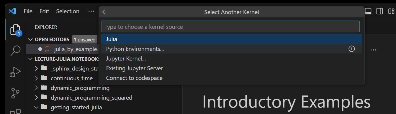
Choose the Julia kernel, rather than the Jupyter Kernel... to bypass the Python Jupyter setup. If successful, you will see the kernel name as Julia channel or something similar.
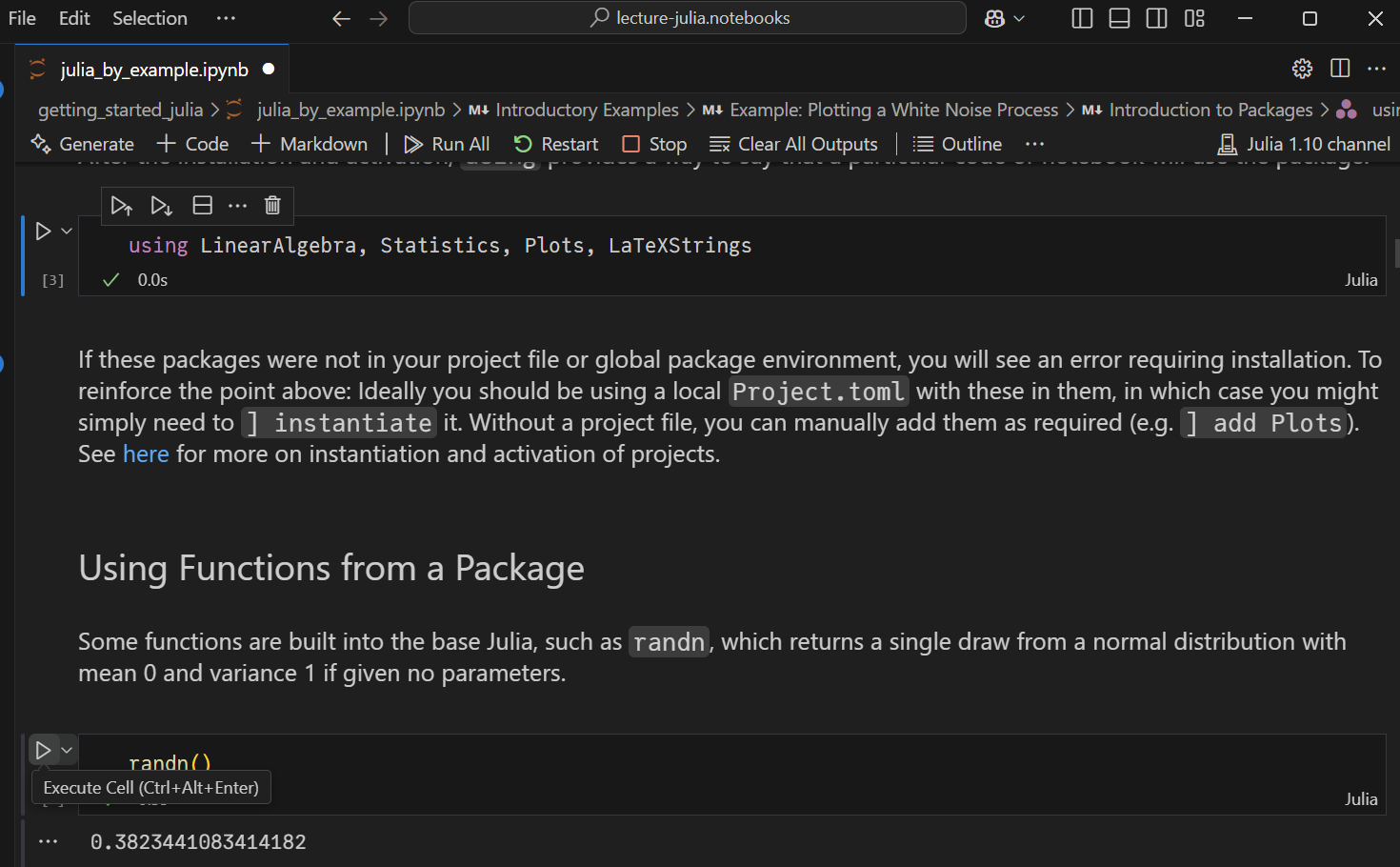
With the kernel selected, you will be able to run cells in the VS Code UI with similar features to Jupyter Lab. For example, below shows the results of play icon next to a code cell, which will Execute Cell and display the results inline.
1.12. Running on Google Colab#
Google Colab provides a hosted Julia runtime that can run the lecture notebooks directly in your browser with no local installation.
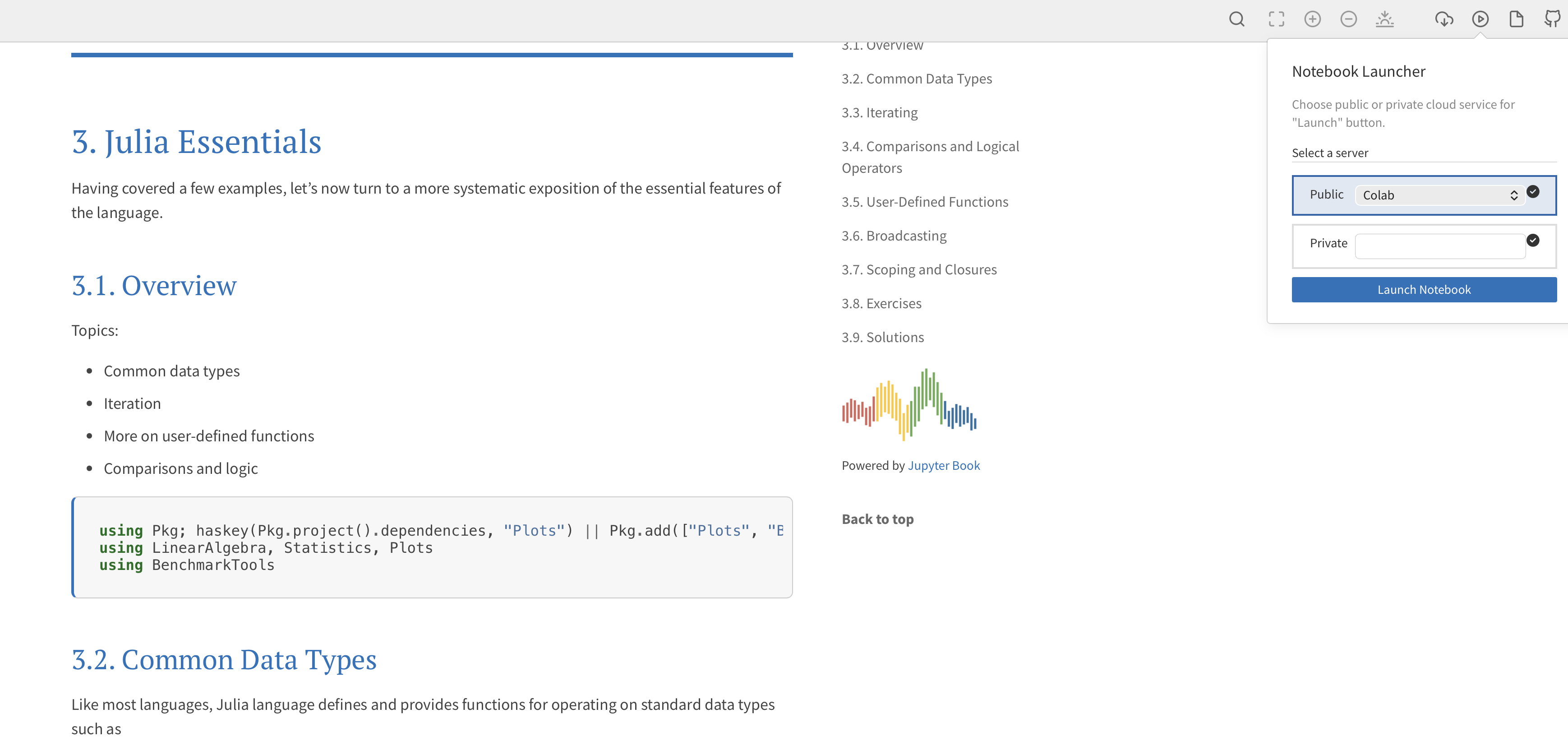
The easiest way to launch any lecture notebook in Colab is to click the icon at the top of the page and select Colab from the Notebook Launcher:
Alternatively, you can navigate to the notebook repository and download or copy the URL. Then log in to colab.research.google.com and choose File > Open notebook > GitHub or the Upload tab to open the notebook.
Once the notebook is open in Colab:
Colab should automatically detect the Julia kernel
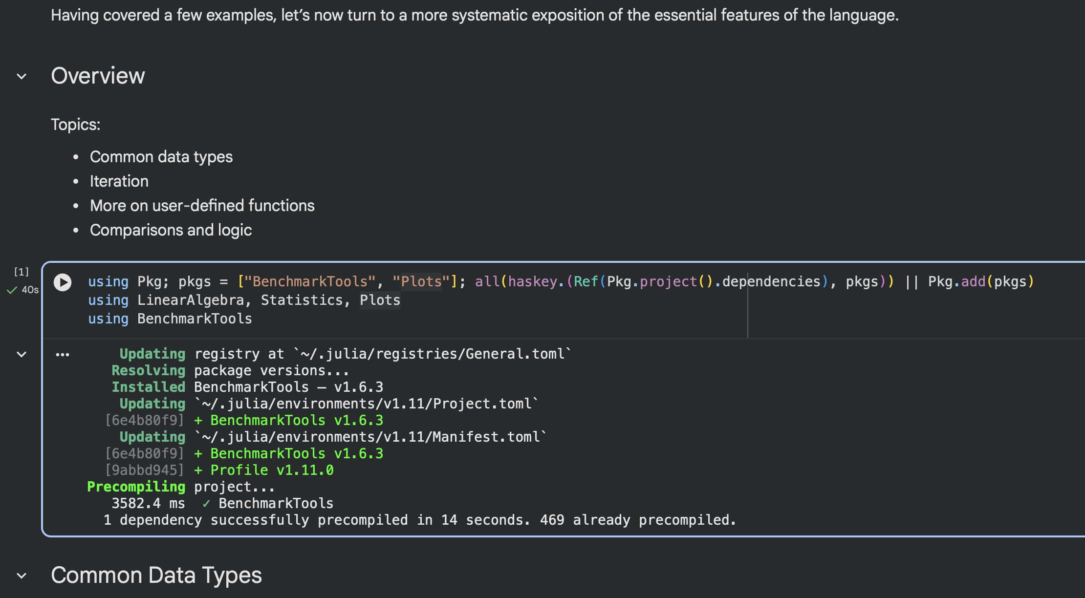
At the top of the first code cell there is a
using Pkg; ... all(haskey.(Ref(Pkg.project().dependencies), pkgs)) || Pkg.add(pkgs)cell to install the required packages after first checking if packages are already installed.Run this cell or the entire notebook to install the packages in the Colab environment. It will be very slow the first time.
After installation completes, the code checks if a key package is already installed, and then will be instantaneous otherwise.
Colab isolates the environment of each notebook, so you will need to run this cell in each notebook you open. However, once the packages are installed in a notebook it may be available when you open the same notebook again in the future.
If there are errors or warnings, then there may be package incompatibilities with the latest released packages. In that case, go back to the traditional method of using a Project.toml and Manifest.toml with the instantiate command.